12.5. Plotting Grid-Relative Wind Barbs

This notebook demonstrates plotting grid-relative wind components as wind barbs along with contours. We’ll continue to use 500-hPa as an example level for plotting purposes.

Grid-Relative Wind Barbs

Unlike observation data, wind components can be stored in two different ways: 1) Earth relative or 2) grid relative. The most common way for the wind components to be stored would be as Earth relative, meaning that the winds are stored in what would be considered the “common” way on a rectilinear grid and would be comparable tp standard observation data. Grid-relative means that the compnents are stored relative to a particular grid projection. Currently the two datasets that have wind components often stored in this grid-relative manner are the North American Model (NAM) and the North American Regional Reanalysis (NARR), whose grid was based off of a historic NAM grid. However, they may not always be stored that way, so you should ALWAYS pay close attention to the meta data associated with your dataset and ensuring the plotted winds conform to known meteorological relationships (e.g., geostrophic/gradient wind balance).

This notebook will demonstrate how MetPy can convert grid-relative winds to be appropriate for your chosen map projection.

Import Packages

Here we bring in the needed Python modules to be able to plot contours using the computer. Note that there are fewer needed for this particular plotting scenario.

from datetime import datetime, timedelta, time, UTC

from metpy.plots import declarative
from metpy.units import units
import xarray as xr

Get Data

Here we are using current data to demonstrate contour plotting with wind barbs. If you have a different data source you would like to use, simply change out the call to remote data in the open_dataset function to be appropriate for the local or remote data you would like to access. Future chapters will demonstrate different data sources that can be commonly used. Here we’ll use the NAM data from the Unidata THREDDS server to demonstrate a dataset that stores grid-relative winds.

# Set the date/time of the model run
# The following code will get you yesterday at 12 UTC
yesterday = datetime.now(UTC) - timedelta(days=1)
model_run_date = datetime.combine(yesterday, time(12))

# Remote access to the NAM dataset from the UCAR site
ds = xr.open_dataset('https://thredds.ucar.edu/thredds/dodsC/grib'
                     f'/NCEP/NAM/CONUS_12km/NAM_CONUS_12km_'
                     f'{model_run_date:%Y%m%d}_{model_run_date:%H%M}.grib2')

Plot Data

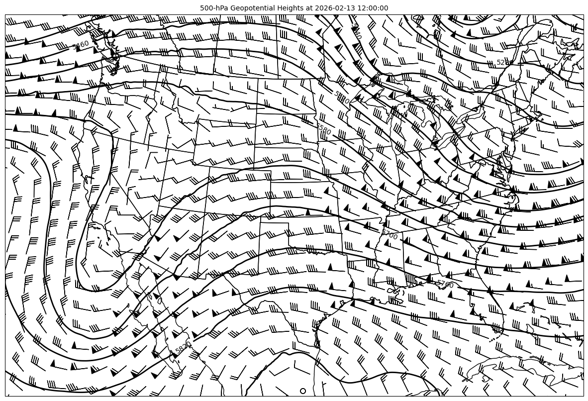
Here we plot the 500-hPa geopotential height and wind barbs for the model initialization time. Once the map in created, look closely at the winds.

# Set the plot time with forecast hours
plot_time = model_run_date + timedelta(hours=0)

# Set attributes for plotting contours
cntr = declarative.ContourPlot()
cntr.data = ds
cntr.field = 'Geopotential_height_isobaric'
cntr.level = 500 * units.hPa
cntr.time = plot_time
cntr.contours = range(0, 10000, 60)
cntr.clabels = True

# Add wind barbds
barbs = declarative.BarbPlot()
barbs.data = ds
barbs.time = plot_time
barbs.field = ['u-component_of_wind_isobaric',
               'v-component_of_wind_isobaric']
barbs.level = 500 * units.hPa
barbs.skip = (15, 15)
barbs.plot_units = 'knot'

# Set the attributes for the map
# and put the contours on the map
panel = declarative.MapPanel()
panel.area = [-125, -74, 22, 52]
panel.projection = 'lcc'
panel.layers = ['states', 'coastline', 'borders']
panel.title = f'500-hPa Geopotential Heights at {plot_time}'
panel.plots = [cntr, barbs]

# Set the attributes for the panel
# and put the panel in the figure
pc = declarative.PanelContainer()
pc.size = (15, 15)
pc.panels = [panel]

# Show the figure
pc.show()

Questions

• What do you notice about the winds?

  • The winds should follow geostrophic/gradient wind balance at this level.

• If you are noticing any issues, look toward the upper-left portion of the map…should the winds be crossing the geopotential heights?

Converting Grid-Relative Winds

In the declarative syntax of MetPy, there is a simple attribute that can be reset to convert the native grid-relative winds to be converted to the appropriate winds for your projection. The parameter on the wind barb class is earth_relative and is a Boolean, which for grid-relative data needs to be set to False. For more details about the settings for plotting gridded data wind barbs checkout the attribute descriptions or head to the MetPy BarbPlot Documentation

# Set the plot time with forecast hours
plot_time = model_run_date + timedelta(hours=0)

# Set attributes for plotting contours
cntr = declarative.ContourPlot()
cntr.data = ds
cntr.field = 'Geopotential_height_isobaric'
cntr.level = 500 * units.hPa
cntr.time = plot_time
cntr.contours = range(0, 10000, 60)
cntr.clabels = True

# Add wind barbds
barbs = declarative.BarbPlot()
barbs.data = ds
barbs.time = plot_time
barbs.field = ['u-component_of_wind_isobaric',
               'v-component_of_wind_isobaric']
barbs.level = 500 * units.hPa
barbs.skip = (15, 15)
barbs.plot_units = 'knot'
barbs.earth_relative = False

# Set the attributes for the map
# and put the contours on the map
panel = declarative.MapPanel()
panel.area = [-125, -74, 22, 52]
panel.projection = 'lcc'
panel.layers = ['states', 'coastline', 'borders']
panel.title = f'500-hPa Geopotential Heights at {plot_time}'
panel.plots = [cntr, barbs]

# Set the attributes for the panel
# and put the panel in the figure
pc = declarative.PanelContainer()
pc.size = (15, 15)
pc.panels = [panel]

# Show the figure
pc.show()

Notice that in the above image, the wind barbs correspond much, MUCH better to geostrophic/gradient wind balance. Even though there is not a lot of change in the middle of the project (this is the result of the projection of the data and the map not being too different), that small difference gets bigger when the projection is more highly curved, which happens toward the edge of the map.

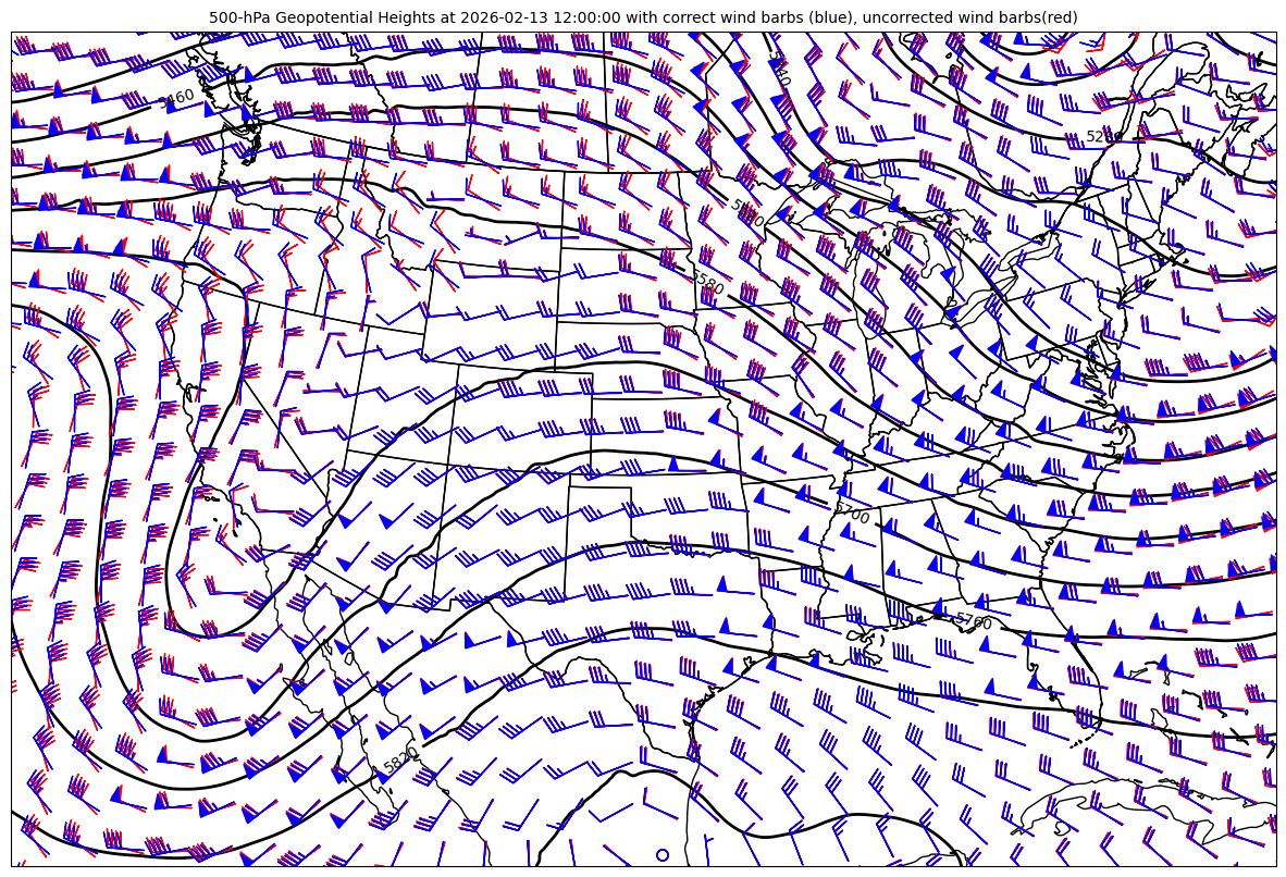
Direct Wind Barb Comparison

Let’s take a look at the two version of the wind barbs, the uncorrected wind barbs are in red in the image below and the re-gridded barbs are plotted in blue.

# Set the plot time with forecast hours
plot_time = model_run_date + timedelta(hours=0)

# Set attributes for plotting contours
cntr = declarative.ContourPlot()
cntr.data = ds
cntr.field = 'Geopotential_height_isobaric'
cntr.level = 500 * units.hPa
cntr.time = plot_time
cntr.contours = range(0, 10000, 60)
cntr.clabels = True

# Add wind barbds
barbs = declarative.BarbPlot()
barbs.data = ds
barbs.time = plot_time
barbs.field = ['u-component_of_wind_isobaric',
               'v-component_of_wind_isobaric']
barbs.level = 500 * units.hPa
barbs.skip = (15, 15)
barbs.plot_units = 'knot'
barbs.earth_relative = False
barbs.color = 'blue'

# Add uncorrected wind barbds
barbs2 = declarative.BarbPlot()
barbs2.data = ds
barbs2.time = plot_time
barbs2.field = ['u-component_of_wind_isobaric',
               'v-component_of_wind_isobaric']
barbs2.level = 500 * units.hPa
barbs2.skip = (15, 15)
barbs2.plot_units = 'knot'
barbs2.color = 'red'

# Set the attributes for the map
# and put the contours on the map
panel = declarative.MapPanel()
panel.area = [-125, -74, 22, 52]
panel.projection = 'lcc'
panel.layers = ['states', 'coastline', 'borders']
panel.title = f'500-hPa Geopotential Heights at {plot_time} with correct wind barbs (blue), uncorrected wind barbs(red)'
panel.plots = [cntr, barbs2, barbs]

# Set the attributes for the panel
# and put the panel in the figure
pc = declarative.PanelContainer()
pc.size = (15, 15)
pc.panels = [panel]

# Show the figure
pc.show()