8.7. Full Surface Station Model Plotting

Import

Import the needed modules

from datetime import datetime, timedelta
from io import StringIO
from urllib.request import urlopen

from metpy.io import metar
from metpy.plots import declarative
from metpy.units import units
import pandas as pd

Read Data

Here we gain access to surface data from the Iowa State Archive. To do so we construct the appropriate data_url that requires a start and end date. To create that we utilize the time we desire and add/subtract time from there to create a time window. From there we use the Pandas module method read_csv() to read in all of the data, then parse the METAR observations using MetPy.

date = datetime(2022, 1, 4, 12)

# Remote Access - Archive Data Read with pandas from Iowa State Archive,
# note differences from METAR files
dt = timedelta(minutes=15)
sdate = date - dt
edate = date + dt
data_url = ('http://mesonet.agron.iastate.edu/cgi-bin/request/asos.py?'
            'data=all&tz=Etc/UTC&format=comma&latlon=yes&'
            f'year1={sdate.year}&month1={sdate.month}&day1={sdate.day}'
            f'&hour1={sdate.hour}&minute1={sdate.minute}&'
            f'year2={edate.year}&month2={edate.month}&day2={edate.day}'
            f'&hour2={edate.hour}&minute2={edate.minute}')
data = pd.read_csv(data_url, skiprows=5, na_values=['M'],
                   low_memory=False).replace('T', 0.00001).groupby('station').tail(1)
df = metar.parse_metar_file(StringIO('\n'.join(val for val in data.metar)),
                            year=date.year, month=date.month)
df['date_time'] = date

df['tmpf'] = (df.air_temperature.values * units.degC).to('degF')
df['dwpf'] = (df.dew_point_temperature.values * units.degC).to('degF')

Plot Data

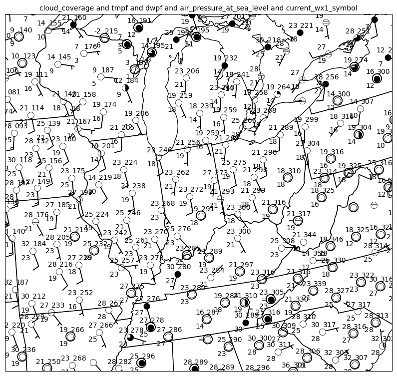
Here we exploit the full range of observations to plot around our station model to get a “full” surface station plot. In order to plot cloud cover and the current weather, we must use the formats to specify the “font” to use, which is part of MetPy. We could go further and change colors, fontsize, etc., but that is left as an excercise for the reader.

mslp_formatter = lambda v: format(v*10, '.0f')[-3:]

# Plot desired data
obs = declarative.PlotObs()
obs.data = df
obs.time = date
obs.time_window = timedelta(minutes=15)
obs.level = None
obs.fields = ['cloud_coverage', 'tmpf', 'dwpf',
              'air_pressure_at_sea_level', 'current_wx1_symbol']
obs.locations = ['C', 'NW', 'SW', 'NE', 'W']
obs.formats = ['sky_cover', None, None, mslp_formatter, 'current_weather']
obs.reduce_points = 0.75
obs.vector_field = ['eastward_wind', 'northward_wind']

# Panel for plot with Map features
panel = declarative.MapPanel()
panel.layout = (1, 1, 1)
panel.projection = 'lcc'
panel.area = 'in'
panel.layers = ['states']
panel.plots = [obs]

# Bringing it all together
pc = declarative.PanelContainer()
pc.size = (10, 10)
pc.panels = [panel]

pc.show()