12.4. Contour Plotting with Wind Barbs

This notebook demonstrates plotting gridded data wind components as wind barbs along with contours. We’ll continue to use 500-hPa as an example level for plotting purposes.

Import Packages

Here we bring in the needed Python modules to be able to plot contours using the computer. Note that there are fewer needed for this particular plotting scenario.

from datetime import datetime, timedelta, time

from metpy.plots import declarative
from metpy.units import units
import xarray as xr

Get Data

Here we are using current data to demonstrate contour plotting with wind barbs. If you have a different data source you would like to use, simply change out the call to remote data in the open_dataset function to be appropriate for the local or remote data you would like to access. Future chapters will demonstrate different data sources that can be commonly used. Here we’ll use the GFS data from the Unidata THREDDS server.

# Set the date/time of the model run
# The following code will get you yesterday at 12 UTC
yesterday = datetime.utcnow() - timedelta(days=1)
model_run_date = datetime.combine(yesterday, time(12))

# Remote access to the dataset from the UCAR site
ds = xr.open_dataset('https://thredds.ucar.edu/thredds/dodsC/grib'
                     f'/NCEP/GFS/Global_onedeg/GFS_Global_onedeg_'
                     f'{model_run_date:%Y%m%d}_{model_run_date:%H%M}.grib2')

# Subset data to be just over the U.S. for plotting purposes
ds = ds.sel(lat=slice(70,10), lon=slice(360-140, 360-60))

Plot Data

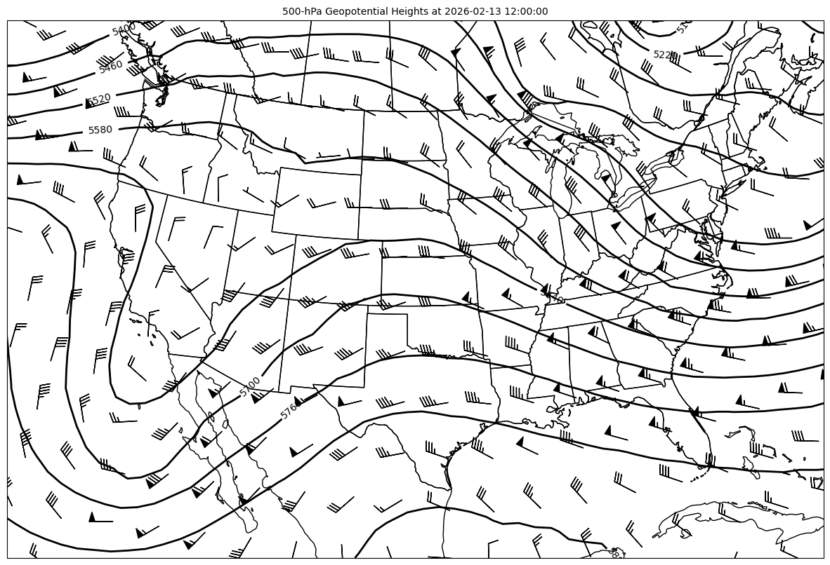
Here we demonstrate the use of BarbPlot(), in addition to still plotting contours of geopotential height, for plotting a vector from its components. For more details about all of the settings for plotting gridded data wind barbs checkout the attribute descriptions or head to the MetPy BarbPlot Documentation

# Set the plot time with forecast hours
plot_time = model_run_date + timedelta(hours=0)

# Set attributes for plotting contours
cntr = declarative.ContourPlot()
cntr.data = ds
cntr.field = 'Geopotential_height_isobaric'
cntr.level = 500 * units.hPa
cntr.time = plot_time
cntr.contours = range(0, 10000, 60)
cntr.clabels = True

# Add wind barbds
barbs = declarative.BarbPlot()
barbs.data = ds
barbs.time = plot_time
barbs.field = ['u-component_of_wind_isobaric',
               'v-component_of_wind_isobaric']
barbs.level = 500 * units.hPa
barbs.skip = (3, 3)
barbs.plot_units = 'knot'

# Set the attributes for the map
# and put the contours on the map
panel = declarative.MapPanel()
panel.area = [-125, -74, 22, 52]
panel.projection = 'lcc'
panel.layers = ['states', 'coastline', 'borders']
panel.title = f'500-hPa Geopotential Heights at {plot_time}'
panel.plots = [cntr, barbs]

# Set the attributes for the panel
# and put the panel in the figure
pc = declarative.PanelContainer()
pc.size = (15, 15)
pc.panels = [panel]

# Show the figure
pc.show()