20.6. Visulalizing and Calculating Parameters on a Skew-T

A powerful tool is being developed that will have the same functionality as GEMPAK, but be done in the Python programming langauage. One example of this is the ability to plot Skew-Ts using the Python module MetPy(). However, there is greatly functionality than that contained in GEMPAK, as you can use MetPy to calculate a whole host of variables from the data plotted on the Skew-T (e.g., CAPE, CIN, LCL, LFC, EL). This notebook is a brief introduction to how that can be done.

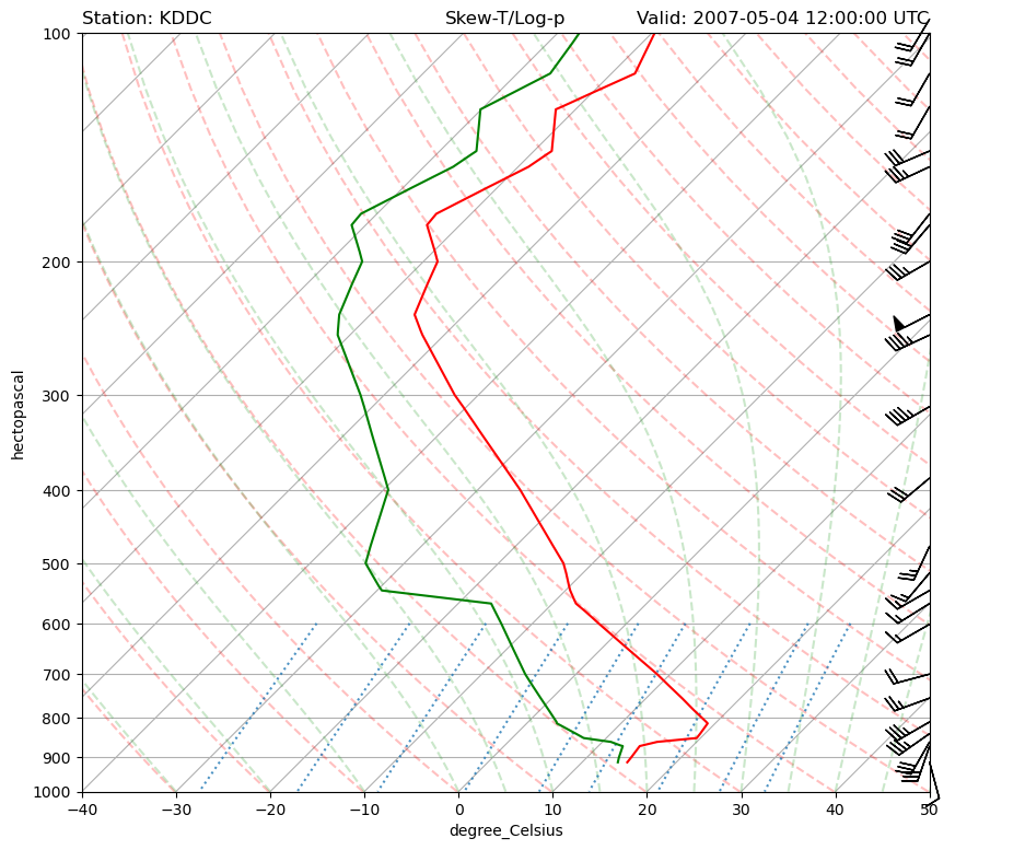
To plot a skew-T, you need to specify the date and time (in UTC) and choose an upper-air station location. The locations of current sounding sites can be found at http://weather.rap.ucar.edu/upper

Import Packages

Here we have a slightly different set of imports to be able to generate a skewT in Python. Here we bring in the SkewT class, a unit helper function and Siphon for reading data from the Wyoming archive.

from datetime import datetime

import matplotlib.pyplot as plt
from metpy.plots import SkewT
from metpy.units import units, pandas_dataframe_to_unit_arrays
import numpy as np
from siphon.simplewebservice.wyoming import WyomingUpperAir

Get Data

Here we will obtain data for a single time for a single station from the Wyoming sounding archive.

https://weather.uwyo.edu/upperair/sounding.html

This dataset is prefered over the Iowa State archive due to how the data come in more ideal for plotting a profile.

# Set date that you want
# Data goes back to the 1970's
date = datetime(2007, 5, 4, 12)

# Set station ID, there are different stations back in the day
# Current station IDs found at http://weather.rap.ucar.edu/upper
station = 'DDC'

# Use Siphon module to grab data from remote server
df = WyomingUpperAir.request_data(date, station)

The data coming from Siphon will be in a Pandas dataframe format, but to use this data with MetPy calculations, we’ll want them as unit arrays. Luckily for us, there is a simple function that we can feed our data object into to get back a dictionary of unit arrays. Below we do that and then subsequently pull out our needed data into separate variables.

# Create dictionary of unit arrays
data = pandas_dataframe_to_unit_arrays(df)

# Isolate united arrays from dictionary to individual variables
p = data['pressure']
T = data['temperature']
Td = data['dewpoint']
u = data['u_wind']
v = data['v_wind']

Now we are ready to use the data for calculation and/or plotting purposes. To begin, we’ll just use the data to make a simple skew-T/log-p diagram plot.

Plot Skew-T

Our plotting is a little different from the syntax we have been using to this point; however, what I hope is that it is pretty simple to understand. First, we create out figure instance, second set up our plot axis (skew), and then we plot on that axis (skew.plot and skew.plot_barbs).

MetPy Skew-T Documentation

# Plot a skew-T image
fig = plt.figure(figsize=(10, 10))

# Set up the skewT axes
skew = SkewT(fig, rotation=45)

# Plot the data using normal plotting functions, in this case using
# log scaling in Y, as dictated by the typical meteorological plot
skew.plot(p, T, 'r')
skew.plot(p, Td, 'g')

# Plot wind barbs, skipping every other one
skew.plot_barbs(p[::2], u[::2], v[::2], y_clip_radius=0.03)

# Set sensible axis limits
skew.ax.set_ylim(1000, 100)
skew.ax.set_xlim(-40, 50)

# Add the relevant special lines
skew.plot_dry_adiabats(t0=np.arange(233,555,10)*units.K, alpha=0.25)
skew.plot_moist_adiabats(colors='tab:green', alpha=0.25)
skew.plot_mixing_lines(colors='tab:blue', linestyle='dotted')

# Plot some titles
plt.title(f'Station: K{station}', loc='left')
plt.title('Skew-T/Log-p', loc='center')
plt.title(f'Valid: {date} UTC', loc='right')

# Show the plot
plt.show()

# Save the plot by uncommenting the following line
#plt.savefig('skewt_image.png', bbox_inches='tight', dpi=150)

This is a bit more of “raw” coding with setting up the figure, axis, and title, but not too much of a stretch from what we were doing before. To save a figure now you use plt.savefig(), but you use the same settings as before.