19.7. Wind Speed Calculation

This notebook demonstrates using a MetPy calculation function to compute a wind speed, save it as a new varaible, and add it to the Dataset for plotting purposes.

Import Packages

from datetime import datetime, timedelta, time

import metpy.calc as mpcalc
from metpy.plots import declarative
from metpy.units import units
import xarray as xr

Get Data

# Set the date/time of the model run for yesterday at 00 UTC
yesterday = datetime.utcnow() - timedelta(days=1)
date = datetime.combine(yesterday, time(0))

# Remote access to the dataset from the UCAR site
ds = xr.open_dataset('https://thredds.ucar.edu/thredds/dodsC/grib/NCEP/GFS/'
                     f'Global_0p5deg_ana/GFS_Global_0p5deg_ana_{date:%Y%m%d_%H}00.grib2')

# Set the plot time
plot_time = date + timedelta(hours=0)

# Subset data to be just over the U.S. for plotting purposes and for the plot_time
ds = ds.metpy.sel(lat=slice(70,10), lon=slice(360-140, 360-60))

Perform Calculation

1. Do the calculation using MetPy (not too hard).

2. Add it to the dataarray.

All MetPy Calculations can be found at https://unidata.github.io/MetPy/latest/api/generated/metpy.calc.html

Not all calculations work on grids, yet!

Wind Speed Calculation in MetPy

We can add a new variable based on a simialr one, then update the values based on the calculation. This is easy for wind speed as it is a variant on a single component of the wind.

# Isolate needed variables for calculations
uwnd = ds['u-component_of_wind_isobaric'].metpy.sel(time=plot_time)
vwnd = ds['v-component_of_wind_isobaric'].metpy.sel(time=plot_time)

# Calculate Wind Speed, store in Dataset
ds['wind_speed'] = mpcalc.wind_speed(uwnd, vwnd)

Plot Data

# Set attributes for plotting contours
cfill = declarative.FilledContourPlot()
cfill.data = ds
cfill.field = 'wind_speed'
cfill.level = 300 * units.hPa
cfill.time = None # We subset for time already
cfill.contours = list(range(10, 201, 20))
cfill.colormap = 'BuPu'
cfill.colorbar = 'horizontal'
cfill.plot_units = 'knot'

cntr2 = declarative.ContourPlot()
cntr2.data = ds
cntr2.field = 'Geopotential_height_isobaric'
cntr2.level = 300 * units.hPa
cntr2.time = plot_time
cntr2.contours = list(range(0, 10000, 120))
cntr2.linecolor = 'black'
cntr2.linestyle = 'solid'
cntr2.clabels = True
cntr2.smooth_field = 4

# Set the attributes for the map
# and put the contours on the map
panel = declarative.MapPanel()
panel.area = [-125, -74, 22, 52]
panel.projection = 'lcc'
panel.layers = ['states', 'coastline', 'borders']
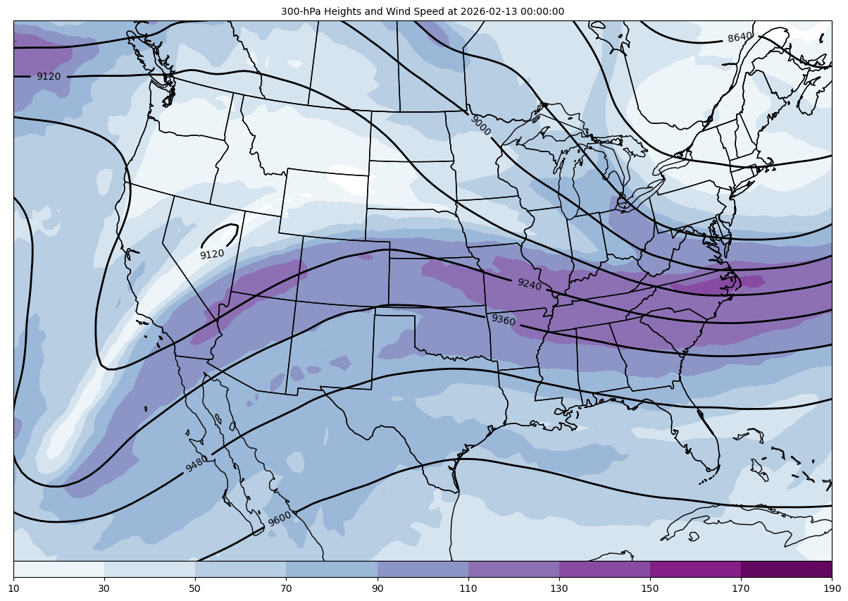
panel.title = f'{cfill.level.m}-hPa Heights and Wind Speed at {plot_time}'
panel.plots = [cfill, cntr2]

# Set the attributes for the panel
# and put the panel in the figure
pc = declarative.PanelContainer()
pc.size = (15, 15)
pc.panels = [panel]

# Show the figure
pc.show()