16.1. Overlay Observations and Contours

Using the declarative syntax to plot upperair observations and overlay contours.

Import Packages

Here we’ll need to import all of the packages to read both observation data and some form of gridded data. Here we’ll plot some upperair maps, so we’ll read current observations from Iowa State archive with current GFS model output to have the computer draw contours.

from datetime import datetime, timedelta, time

import cartopy.crs as ccrs
from metpy.io import add_station_lat_lon
from metpy.plots import declarative
from metpy.units import units
import numpy as np
from siphon.simplewebservice.iastate import IAStateUpperAir
import xarray as xr

Get Observations Data

Here we’ll get the observation data from the Iowa State archive, add some latitude/longitude data to those observations and remove an errant data point that got tagged as ‘KVER’.

# Set the date/time of the model run
# The following code will get you yesterday at 12 UTC
yesterday = datetime.utcnow() - timedelta(days=1)
date = datetime.combine(yesterday, time(12))

# Request data using Siphon request for data from Iowa State Archive
data = IAStateUpperAir.request_all_data(date)

# Add lat/lon information to dataframe, drop missing station lat/lons
df = add_station_lat_lon(data, data.station.name).dropna(subset=['latitude', 'longitude'])
df = df[df.station != 'KVER']

Downloading file 'sfstns.tbl' from 'https://github.com/Unidata/MetPy/raw/v1.6.3/staticdata/sfstns.tbl' to '/Users/kgoebber/Library/Caches/metpy/v1.6.3'.

Downloading file 'master.txt' from 'https://github.com/Unidata/MetPy/raw/v1.6.3/staticdata/master.txt' to '/Users/kgoebber/Library/Caches/metpy/v1.6.3'.

Downloading file 'stations.txt' from 'https://github.com/Unidata/MetPy/raw/v1.6.3/staticdata/stations.txt' to '/Users/kgoebber/Library/Caches/metpy/v1.6.3'.

Downloading file 'airport-codes.csv' from 'https://github.com/Unidata/MetPy/raw/v1.6.3/staticdata/airport-codes.csv' to '/Users/kgoebber/Library/Caches/metpy/v1.6.3'.

Get Gridded Data

Here we’ll get the associated gridded output to be able to draw contours from Unidata. Here we use the one degree GFS output.= and subset to being over the CONUS.

# Get GFS data for contouring
ds = xr.open_dataset('https://thredds.ucar.edu/thredds/dodsC/grib/NCEP/GFS/'
                     f'Global_onedeg_ana/GFS_Global_onedeg_ana_{date:%Y%m%d_%H%M}.grib2')

# Subset data to be just over the CONUS
ds = ds.sel(lat=slice(80, 10), lon=slice(360-140, 360-40))

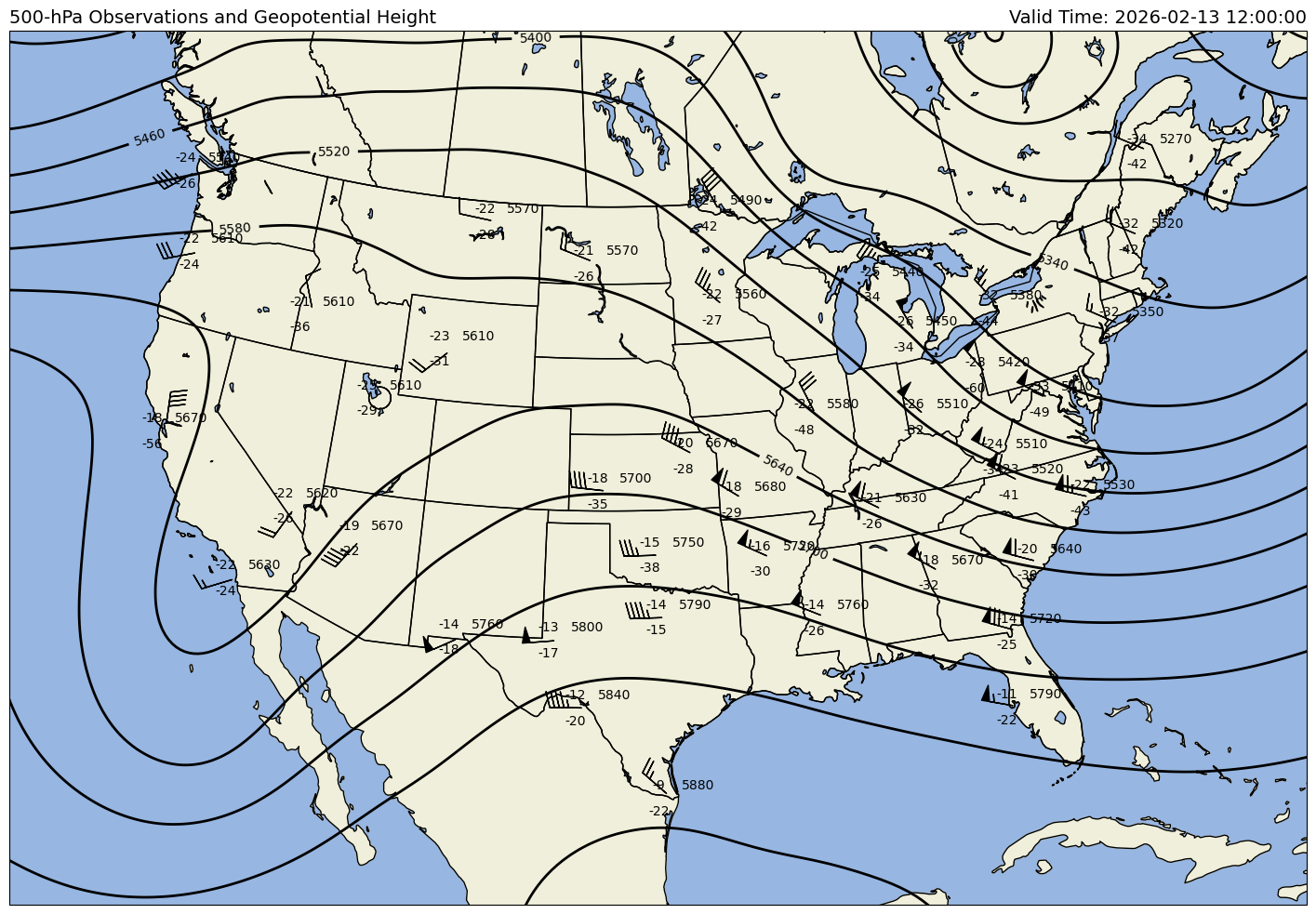
Plot Obs and Contours

To plot our overlay all we need to do is set up both our attributes for plotting the observations and for drawing contours, then add both pieces and put it on a map figure.

# Add point observations
obs = declarative.PlotObs()
obs.data = df
obs.level = 500 * units.hPa
obs.time = date
obs.fields = ['temperature', 'dewpoint', 'height']
obs.locations = ['NW', 'SW', 'ENE']
obs.vector_field = ['u_wind', 'v_wind']
obs.vector_field_length = 7

# Add contours of geopotential height
cntr = declarative.ContourPlot()
cntr.data = ds
cntr.level = obs.level
cntr.time = date
cntr.field = 'Geopotential_height_isobaric'
cntr.clabels = True
cntr.contours = range(0, 10000, 60)
cntr.smooth_field = 3
cntr.smooth_contour = 5

# Set map panel features
panel = declarative.MapPanel()
panel.projection = 'lcc'
panel.area = [-124, -72, 22, 53]
panel.layers = ['ocean', 'lakes', 'land', 'states', 'borders', 'coastline']
panel.left_title = f'{obs.level.m}-hPa Observations and Geopotential Height'
panel.right_title = f'Valid Time: {date}'
panel.title_fontsize = 14
panel.plots = [cntr, obs]

# Add map panel to figure
pc = declarative.PanelContainer()
pc.size = (18, 18)
pc.panels = [panel]

pc.show()