8.4. Surface Data and Plotting using MetPy

This notebook demonstrates reading surface data and plotting it using MetPy’s declarative syntax.

To make a plot of surface observations requires three elements

• PlotObs() to specify the observations to be plotted

• MapPanel() to specify the characteristics of the map to plot the observations on

• PanelContainer() to collect one or more panels.

These three elements are separate parts of the declarative module from MetPy. In Python we call these parts Classes and note that they contain MiXeD case names. These classes contain a number of attributes that can be set to specify what and how to plot the data in a figure. The descriptions of some of the basic elements of each element are given below.

Import Modules

Here we’ll import those modules that are needed to produce read in remote surface METAR observation data, process those observations, and plot the values on a map.

from datetime import datetime, timedelta
from io import StringIO
from urllib.request import urlopen

from metpy.io import metar
from metpy.plots import declarative
from metpy.units import units
import pandas as pd

Read Data

The surface data are in METAR format and store the data files at this location for approximately two weeks.

The format of the filenames are YYYYMMDDHH_sao.wmo where YYYY is the year, MM is the month, DD is the day, and HH is the hour.

date = datetime.utcnow()

# Remote Access - Archive Data Read with pandas from Iowa State Archive,
# note differences from METAR files
dt = timedelta(minutes=30)
sdate = date - dt
edate = date + dt
data_url = ('http://mesonet.agron.iastate.edu/cgi-bin/request/asos.py?'
            'data=all&tz=Etc/UTC&format=comma&latlon=yes&'
            f'year1={sdate.year}&month1={sdate.month}&day1={sdate.day}'
            f'&hour1={sdate.hour}&minute1={sdate.minute}&'
            f'year2={edate.year}&month2={edate.month}&day2={edate.day}'
            f'&hour2={edate.hour}&minute2={edate.minute}')
data = pd.read_csv(data_url, skiprows=5, na_values=['M'],
                   low_memory=False).replace('T', 0.00001).groupby('station').tail(1)
df = metar.parse_metar_file(StringIO('\n'.join(val for val in data.metar)),
                            year=date.year, month=date.month)
# Local Access
# data = f'/data/ldmdata/surface/sao/{date:%Y%m%d%H}_sao.wmo'
# df = metar.parse_metar_file(data, year=date.year, month=date.month)

Plot Data

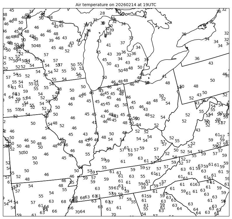
Here we seek to use the data that were just read in to plot the air_temperature variable in units of Fahrenheit. Since surface observations can be associated with a range of times, we can set the time_window attribute to look over a range of times. These temperatures will be plotted on a map over a small geographic location and a title is added to the map.

# Plot desired data
obs = declarative.PlotObs()
obs.data = df
obs.time = date
obs.time_window = timedelta(minutes=30)
obs.fields = ['air_temperature']
obs.plot_units = ['degF']

# Panel for plot with Map features
panel = declarative.MapPanel()
panel.layout = (1, 1, 1)
panel.projection = 'lcc'
panel.area = 'in'
panel.layers = ['states']
panel.title = f'Air temperature on {date:%Y%m%d} at {date:%H}UTC'
panel.plots = [obs]

# Bringing it all together
pc = declarative.PanelContainer()
pc.size = (10, 10)
pc.panels = [panel]

pc.show()

Note

The use of formatted strings (f-strings) are used extensively in this book. Use of these strings allows the easy input of variables into a string value to dynamically generate the string. Variables can also be formatted (depending on type) to gain more control over how the values plot. In the above surface plot, f-strings are used to set the title where we use the variable date with date formatting to make a nice, reable title.

For more information on f-strings, see the Python documentation