21.5. Color-Enhanced Satellite Imagery

To plot satellite imagery we can use data that we bring in through our local data feed or remote access from UCAR. Satellite data are stored in /data/ldmdata/satellite for both GOES-16 and GOES-17 or at https://thredds.ucar.edu/thredds/idd/satellite.html. We’ll be using the remote data source in this notebook. There are a couple of different sectors that we can view the data from, but the most common for synoptic-dynamic purposes would be the CONUS projection. Data are available every 5 min.

For this plotting we are doing to use the declarative plotting syntax using Python and the MetPy module.

Import Packages

from datetime import datetime, UTC

import metpy.calc as mpcalc
from metpy.plots import declarative
from metpy.units import units
import numpy as np
from siphon.catalog import TDSCatalog
import xarray as xr

Get Data

date = datetime.now(UTC).replace(tzinfo=None)

# Create variables for URL generation
region = 'CONUS'
channel = 9
satellite = 'east'

# We want to match something like:
# https://thredds-test.unidata.ucar.edu/thredds/catalog/satellite/goes16/GOES16/Mesoscale-1/Channel08/20181113/catalog.html

# Construct the data_url string
data_url = (f'https://thredds.ucar.edu/thredds/catalog/satellite/goes/{satellite}/'
            f'products/CloudAndMoistureImagery/{region}/Channel{channel:02d}/'
            f'{date:%Y%m%d}/catalog.xml')

# Get list of files available for particular day
cat = TDSCatalog(data_url)

# Grab dataset for desired time
dataset = cat.datasets.filter_time_nearest(date, regex=r'_s(?P<strptime>\d{13})', strptime='%Y%j%H%M%S')

# Open most recent file available
ds = dataset.remote_access(use_xarray=True)

# Apply a square root correction for visible imagery only
if channel == 2:
    ds['Sectorized_CMI'].values = np.sqrt(ds['Sectorized_CMI'].values)

# Grab time from file and make into datetime object for plotting and later data access
vtime = ds.time.values.astype('datetime64[ms]').astype('O')

Plot Imagery

Color enhancement colormaps are available from MetPy and can be found at: https://unidata.github.io/MetPy/latest/api/generated/metpy.plots.ctables.html

Water Vapor Colormaps:

• WVCIMSS_r

• wv_tpc_r

Infrared Colormaps:

• ir_drgb

• ir_tmpc

• ir_rgbv

• ir_bd

Note

The _r can be added to any colormap name to reverse the colormap. Depending on the data you may have to switch between reveresed and non-reveresed colormaps.

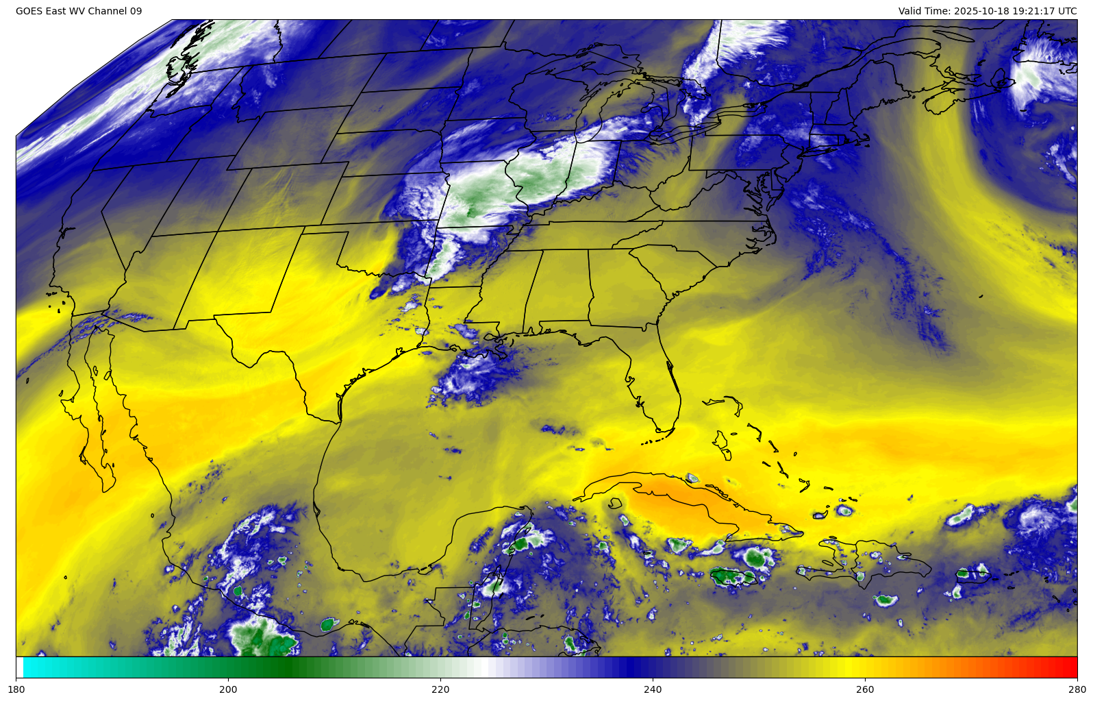
# Declare the data we wish to plot
img = declarative.ImagePlot()
img.data = ds
img.field = 'Sectorized_CMI'
img.colormap = 'WVCIMSS_r'
img.colorbar = 'horizontal'
img.image_range = (180, 280)

# Plot the data on a map
panel = declarative.MapPanel()
panel.layers = ['coastline', 'borders', 'states']
panel.left_title = f'GOES East WV Channel {channel:02d}'
panel.right_title = f'Valid Time: {vtime} UTC'
panel.plots = [img]

# Place the map on a figure
pc = declarative.PanelContainer()
pc.size = (20, 16)
pc.panels = [panel]
#pc.save(f'GOES_East_{vtime:%Y%m%d_%H%M}_colorenhanced.png', bbox_inches='tight', dpi=150)
pc.show()