13.2. Geostrophic Balance

One very common horizontal force balance is the geostrophic balance. Flows in the atmosphere are often over large enough temporal and spatial scales that bring the Coriolis force into play. In the upper-levels (i.e., generally above 700 hPa) when the flow is basically straight (i.e., not strongly curved) the atmosphere can be approximated to be in geostrophic balance. The balance is between the pressure gradient (height gradient) force and the Coriolis force (Fig. 13.2) and can be written algebraically for a constant height surface as,

\[ \begin{align}\begin{aligned} 0 = -\frac{1}{\rho}\frac{\Delta p}{\Delta x} + f v_g\\0 = -\frac{1}{\rho}\frac{\Delta p}{\Delta y} - f u_g \end{aligned}\end{align} \]

where the subscript \(g\) signifies the geostrophic wind. Note how we also choose to separate the wind into \(u_g\) and \(v_g\) components, symbolizing west/east and south/north flow respectively. We can rewrite the right-hand side of the force balance for geopotential height as,

\[ \begin{align}\begin{aligned} 0 = -g\frac{\Delta z}{\Delta x} + f v_g\\0 = -g\frac{\Delta z}{\Delta y} - f u_g \end{aligned}\end{align} \]

where \(g\Delta z = \Delta \Phi\) and is known as geopotential height. Solving for \(v_g\) and \(u_g\) yields an equation for the geostrophic wind on a constant pressure surface,

\[ \begin{align}\begin{aligned} v_g = \frac{g}{f}\frac{\Delta z}{\Delta x}\\u_g = -\frac{g}{f}\frac{\Delta z}{\Delta y} \end{aligned}\end{align} \]

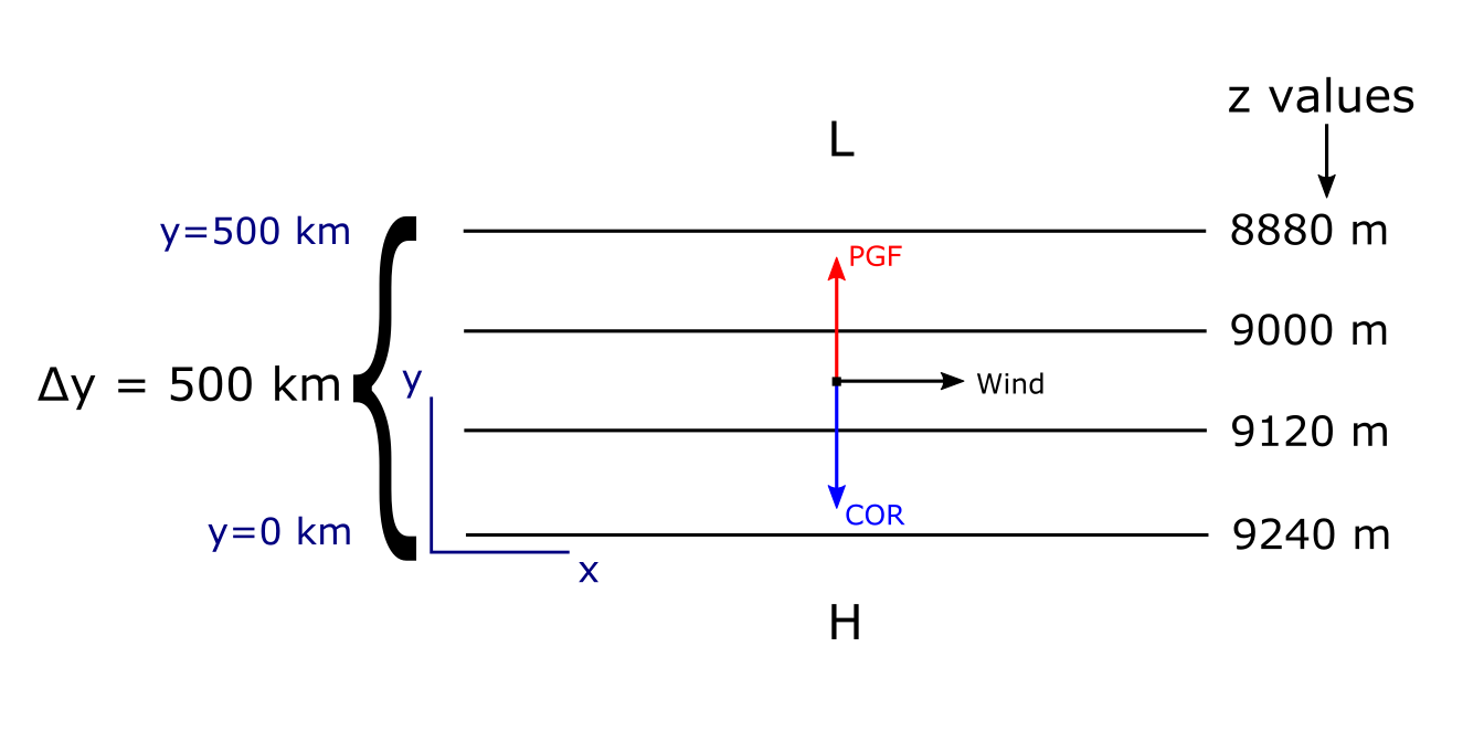
Fig. 13.2 Demonstration of geostrophic balance with example force balance diagram and annotated figure elements.

Example Geostrophic Wind Calculation

Having these equations are great, but what can we do with them? We can use them to calculate the values of the wind components by using the geopotential height gradient, the Coriolis parameter, and the value of gravity. We’ll use the values from the illustration in Figure 13.2 to obtain our values and complete our calculation.

Note

Be careful when setting up calculations to be sure that you are doing your differencing in the same way. If you don’t, then you can end up with a sign error (e.g., a negative when you should be getting a positive).

\(u_g\) Calculation

\[\Delta z\ (\text{y-direction})\ = \ 8880\ m\ - \ 9240\ m\ = \ - 360\ m\]

\[\Delta y\ = \ 500 \cdot 1000\ m\ - \ 0\ m\ = \ 500000\ m\]

\[g = 9.81\ m\ s^{- 2}\]

\[u_{g} = - \frac{9.81\ m\ s^{- 2}}{10^{- 4}\ s^{- 1}}\frac{- 360\ m}{500000\ m} = 70.6\ m\ s^{- 1}\]

\(v_g\) Calculation

\[\Delta z\ (\text{x-direction})\ = \ 9000\ m\ - \ 9000\ m\ = \ 0\ m\]

\[v_{g} = \frac{9.81\ m\ s^{- 2}}{10^{- 4}\ s^{- 1}}\frac{0\ m}{500000\ m} = 0\ m\ s^{- 1}\]

This is because there is no change in the geopotential height values in the x-direction.