19.11. Relative Vorticity Calculation

This notebook demonstrates computing relative vorticity, then plotting it using color-filled contours.

Import Packages

from datetime import datetime, timedelta, time

import metpy.calc as mpcalc
from metpy.plots import declarative
from metpy.units import units
import xarray as xr

Get Data

# Set the date/time of the model run
yesterday = datetime.utcnow() - timedelta(days=1)
model_run_time = datetime.combine(yesterday, time(0))

# Remote access to the dataset from the UCAR site
ds = xr.open_dataset('https://thredds.ucar.edu/thredds/dodsC/grib'
                     f'/NCEP/GFS/Global_onedeg/GFS_Global_onedeg_'
                     f'{model_run_time:%Y%m%d}_{model_run_time:%H%M}.grib2')

# Subset data to be just over the U.S. for plotting purposes
ds = ds.sel(lat=slice(70,10), lon=slice(360-150, 360-55))

Calculation

1. Pull out necessary variables from dataset.

2. Do the calculation using MetPy (not too hard).

3. Add it to the dataarray.

All MetPy Calculations can be found at https://unidata.github.io/MetPy/latest/api/generated/metpy.calc.html

Note

Not all calculations work on grids, yet!

(19.2)\[\begin{align} \text{Relative Vorticity} = \zeta & = \frac{\Delta V}{\Delta x} - \frac{\Delta U}{\Delta y} \\ \end{align}\]

MetPy Relative Vorticity Calculation

# Select Level and Time
level = 500 * units.hPa
plot_time = model_run_time + timedelta(hours=0)

# Isolate needed variables
uwnd = ds['u-component_of_wind_isobaric'].metpy.sel(vertical=level, time=plot_time)
vwnd = ds['v-component_of_wind_isobaric'].metpy.sel(vertical=level, time=plot_time)

# Compute relative vorticity and store in Dataset
ds['relative_vorticity'] = mpcalc.vorticity(uwnd, vwnd)

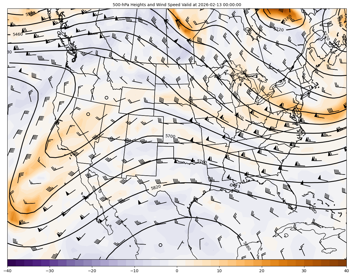
Plot Relative Vorticity

In addition to plotting our newly calculated relative vorticity variable, we’ll smooth the Geopotential Hieghts using the smooth_field attribute.

# Set attributes for plotting contours
cfill = declarative.FilledContourPlot()
cfill.data = ds
cfill.field = 'relative_vorticity'
cfill.level = None
cfill.time = None
cfill.contours = list(range(-40, 41, 2))
cfill.colormap = 'PuOr_r'
cfill.colorbar = 'horizontal'
cfill.scale = 1e5

cntr2 = declarative.ContourPlot()
cntr2.data = ds
cntr2.field = 'Geopotential_height_isobaric'
cntr2.level = 500 * units.hPa
cntr2.time = plot_time
cntr2.contours = list(range(0, 10000, 60))
cntr2.linecolor = 'black'
cntr2.linestyle = 'solid'
cntr2.clabels = True
cntr2.smooth_field = 2

barbs = declarative.BarbPlot()
barbs.data = ds
barbs.time = plot_time
barbs.field = ['u-component_of_wind_isobaric', 'v-component_of_wind_isobaric']
barbs.level = level
barbs.skip = (3, 3)
barbs.plot_units = 'knot'

# Set the attributes for the map
# and put the contours on the map
panel = declarative.MapPanel()
panel.area = [-125, -74, 20, 55]
panel.projection = 'lcc'
panel.layers = ['states', 'coastline', 'borders']
panel.title = f'{cntr2.level.m}-hPa Heights and Wind Speed Valid at {plot_time}'
panel.plots = [cfill, cntr2, barbs]

# Set the attributes for the panel
# and put the panel in the figure
pc = declarative.PanelContainer()
pc.size = (15, 15)
pc.panels = [panel]

# Show the figure
pc.show()