21.3. Satellite Imagery

To plot satellite imagery, we can use the same plotting techniques we have been using all semester to plot gridded data. Satellite data is similar to model output in that each pixel of the image is evenly spaced and can be plotted using the ImagePlot() class from the declarative syntax in MetPy.

Import Packages

Similar to accessing the Iowa State/Wyoming Upperair archive we can use the Python module Siphon to help gain access to the satellite data.

from datetime import datetime, UTC

from metpy.plots import declarative
from metpy.units import units
import numpy as np
from siphon.catalog import TDSCatalog
import xarray as xr

Get Data

We use a set of variables to help construct the web URL including, region, channel, and satellite. This will help us when we simply want to view a slightly different satellite product. After constructing the data_url, then we can use the helper function to find us the right file and use Siphon to grab the correct link to the dataset on the UCAR server. Then we’ll bring that dataset into our notebook and made to look like an xarray data object, which is what we have been working with through all of our model output.

# Set the datetime from the computer
date = datetime.now(UTC).replace(tzinfo=None)

# Create variables for URL generation
region = 'CONUS'
channel = 2
satellite = 'east'

# We want to match something like:
# https://thredds-test.unidata.ucar.edu/thredds/catalog/satellite/goes16/GOES16/Mesoscale-1/Channel08/20181113/catalog.html

# Construct the data_url string
data_url = (f'https://thredds.ucar.edu/thredds/catalog/satellite/goes/{satellite}/'
            f'products/CloudAndMoistureImagery/{region}/Channel{channel:02d}/'
            f'{date:%Y%m%d}/catalog.xml')

# Get list of files available for particular day
cat = TDSCatalog(data_url)

# Grab dataset for desired time
dataset = cat.datasets.filter_time_nearest(date, regex=r'_s(?P<strptime>\d{13})', strptime='%Y%j%H%M%S')

# Open most recent file available
ds = dataset.remote_access(use_xarray=True)

# Apply a square root correction for visible imagery only
if channel == 2:
    ds['Sectorized_CMI'].values = np.sqrt(ds['Sectorized_CMI'].values)

# Grab time from file and make into datetime object for plotting and later data access
vtime = ds.time.values.astype('datetime64[ms]').astype('O')

Plot Imagery

From here, plotting becomes relatively routine, expect we’ll want to use the ImagePlot() class since we are plotting a satellite image. We are going to use the time form the actual file for plotting purposes since we don’t know the exact time of the data we got back from the server.

The files that we are using are called Cloud and Moisture Imagery files. That means that the data have been converted to a format that is more amenable for plotting (either reflectance or brightness temperature). So, the name of the variable we want to plot is 'Sectorized_CMI'.

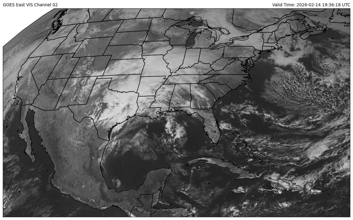
A simple map can then be generated via the following settings using a grey scale image.

# Declare the data we wish to plot
img = declarative.ImagePlot()
img.data = ds
img.field = 'Sectorized_CMI'
img.colormap = 'Greys_r'

# Plot the data on a map
panel = declarative.MapPanel()
panel.layers = ['coastline', 'borders', 'states']
panel.left_title = f'GOES East VIS Channel {channel:02d}'
panel.right_title = f'Valid Time: {vtime} UTC'
panel.plots = [img]

# Place the map on a figure
pc = declarative.PanelContainer()
pc.size = (15, 15)
pc.panels = [panel]
pc.show()