12.6. Plotting Multiple Contours

This notebook demonstrates plotting multiple contours from gridded data. Here we’ll plot 850-hPa geopotential heights with 850-hPa temperature in Celisus.

Import Packages

Here we bring in the needed Python modules to be able to plot contours using the computer. Note that there are fewer needed for this particular plotting scenario.

from datetime import datetime, timedelta, time

from metpy.plots import declarative
from metpy.units import units
import xarray as xr

Get Data

Here we are using the same current data that we have used in this chapter from the one degree GFS to demonstrate our plotting.

# Set the date/time of the model run
# The following code will get you yesterday at 12 UTC
yesterday = datetime.utcnow() - timedelta(days=1)
model_run_date = datetime.combine(yesterday, time(12))

# Remote access to the dataset from the UCAR site
ds = xr.open_dataset('https://thredds.ucar.edu/thredds/dodsC/grib'
                     f'/NCEP/GFS/Global_onedeg/GFS_Global_onedeg_'
                     f'{model_run_date:%Y%m%d}_{model_run_date:%H%M}.grib2')

# Subset data to be just over the U.S. for plotting purposes
ds = ds.sel(lat=slice(70,10), lon=slice(360-140, 360-60))

Plot Data

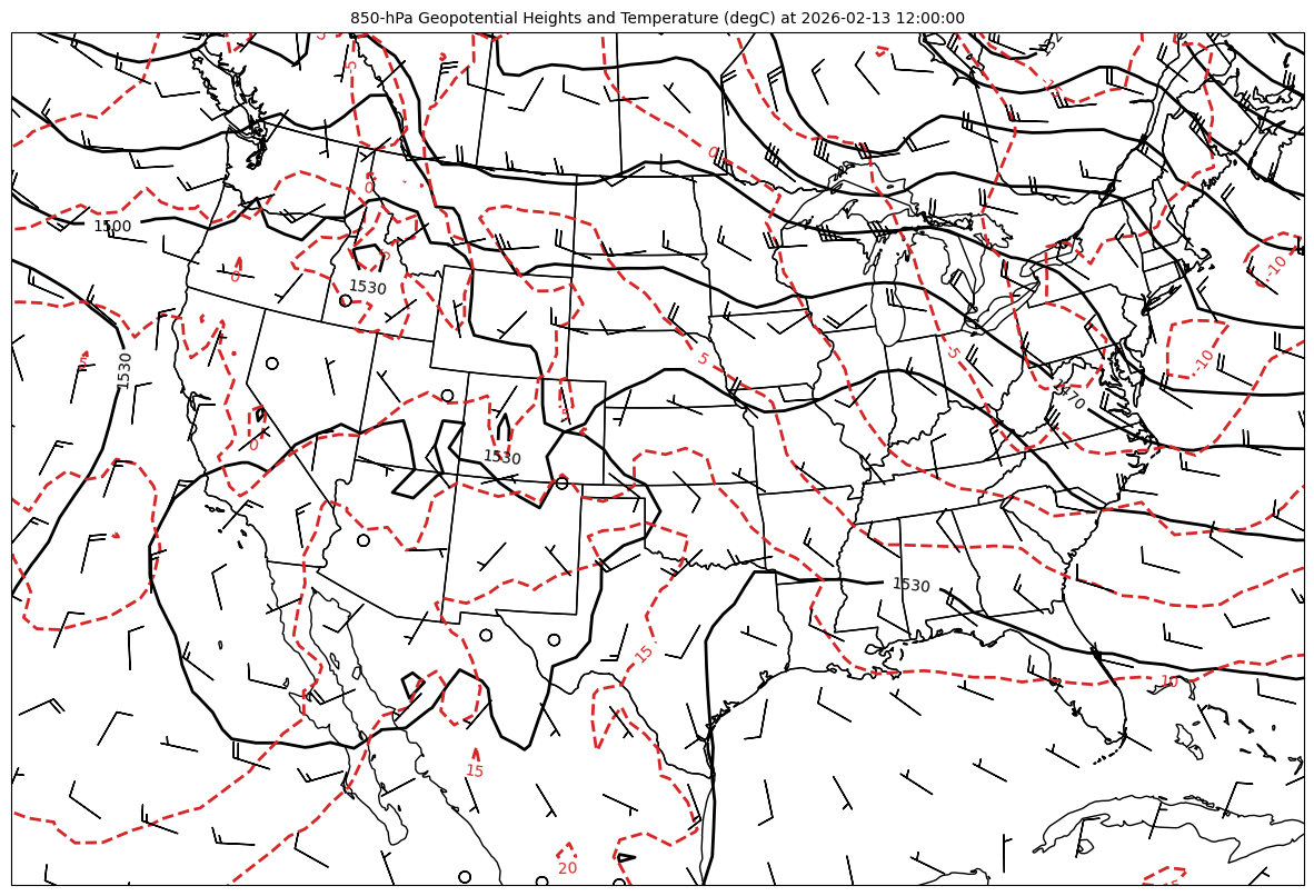
Here we demonstrate how to overlay multiple contours on a single plot (with wind barbs still plotted). You’ll want to be sure you use two unique variable names for each set of contours and set appropriate attributes to have each contour plot just a little differently (e.g., different colors and/or linestyles).

# Set the plot time with forecast hours
plot_time = model_run_date + timedelta(hours=0)

# Set attributes for plotting geopotential height contours
hght = declarative.ContourPlot()
hght.data = ds
hght.field = 'Geopotential_height_isobaric'
hght.level = 850 * units.hPa
hght.time = plot_time
hght.contours = range(0, 10000, 30)
hght.clabels = True

# Set attributes for plotting temperature contours in Celsius
tmpc = declarative.ContourPlot()
tmpc.data = ds
tmpc.field = 'Temperature_isobaric'
tmpc.level = 850 * units.hPa
tmpc.time = plot_time
tmpc.contours = range(-40, 41, 5)
tmpc.clabels = True
tmpc.linestyle = 'dashed'
tmpc.linecolor = 'tab:red'
tmpc.plot_units = 'degC'

# Add wind barbds
barbs = declarative.BarbPlot()
barbs.data = ds
barbs.time = plot_time
barbs.field = ['u-component_of_wind_isobaric',
               'v-component_of_wind_isobaric']
barbs.level = 850 * units.hPa
barbs.skip = (3, 3)
barbs.plot_units = 'knot'

# Set the attributes for the map
# and put the contours on the map
panel = declarative.MapPanel()
panel.area = [-125, -74, 22, 52]
panel.projection = 'lcc'
panel.layers = ['states', 'coastline', 'borders']
panel.title = f'850-hPa Geopotential Heights and Temperature (degC) at {plot_time}'
panel.plots = [hght, tmpc, barbs]

# Set the attributes for the panel
# and put the panel in the figure
pc = declarative.PanelContainer()
pc.size = (15, 15)
pc.panels = [panel]

# Show the figure
pc.show()