19.2. Thickness Calculation

This notebook demonstrates a simple calculation for 1000-500-hPa thickness by adding it to the DataArray.

Import Packages

from datetime import datetime, timedelta

from metpy.plots import declarative
from metpy.units import units
import numpy as np
import xarray as xr

Get Data

# Set the date/time of the model run
date = datetime(2017, 2, 24, 12)

# Remote access to the dataset from the NCEI Archive
ds = xr.open_dataset('https://www.ncei.noaa.gov/thredds/dodsC/model-gfs-g3-anl-files-old'
                     f'/{date:%Y%m}/{date:%Y%m%d}/gfsanl_3_{date:%Y%m%d_%H}00_000.grb')

# Subset data to be just over the U.S. for plotting purposes
ds = ds.sel(lat=slice(70,10), lon=slice(360-140, 360-60))

A Simple Calculation

1000-500-hPa Thickness = (Heights at 500 hPa) - (Heights at 1000 hPa)

Easy to do subtraction with a data array and store it directly back into the dataset (ds). In order to do this well, we’ll need to quantify the variable (e.g., attach units to the variable we’re pulling from our Dataset. Then we’ll do the calculation and dequantify it so we are back in a more native xarray DataArray format.

hght_500 = ds.Geopotential_height_isobaric.metpy.sel(time=date,
    vertical=500 * units.hPa).metpy.quantify()
hght_1000 = ds.Geopotential_height_isobaric.metpy.sel(time=date,
    vertical=1000 * units.hPa).metpy.quantify()
ds['thickness'] = (hght_500 - hght_1000).metpy.dequantify()

Plot Data

Note

Since we subset by time, as well as by vertical level, when isolating the 500 and 1000-hPa geopotential heights above, we no longer need to subst by those dimensions when plotting. So we’ll need to set the level and time attributes to None.

# Set attributes for plotting contours
cntr = declarative.ContourPlot()
cntr.data = ds
cntr.field = 'thickness'
cntr.level = None
cntr.time = None
cntr.contours = list(range(0, 10000, 60))
cntr.linecolor = 'red'
cntr.linestyle = 'dashed'
cntr.clabels = True

cntr2 = declarative.ContourPlot()
cntr2.data = ds
cntr2.field = 'Geopotential_height_isobaric'
cntr2.level = 500 * units.hPa
cntr2.time = date
cntr2.contours = range(0, 10000, 60)
cntr2.linecolor = 'black'
cntr2.linestyle = 'solid'
cntr2.clabels = True

# Set the attributes for the map
# and put the contours on the map
panel = declarative.MapPanel()
panel.area = [-125, -74, 20, 55]
panel.projection = 'lcc'
panel.layers = ['states', 'coastline', 'borders']
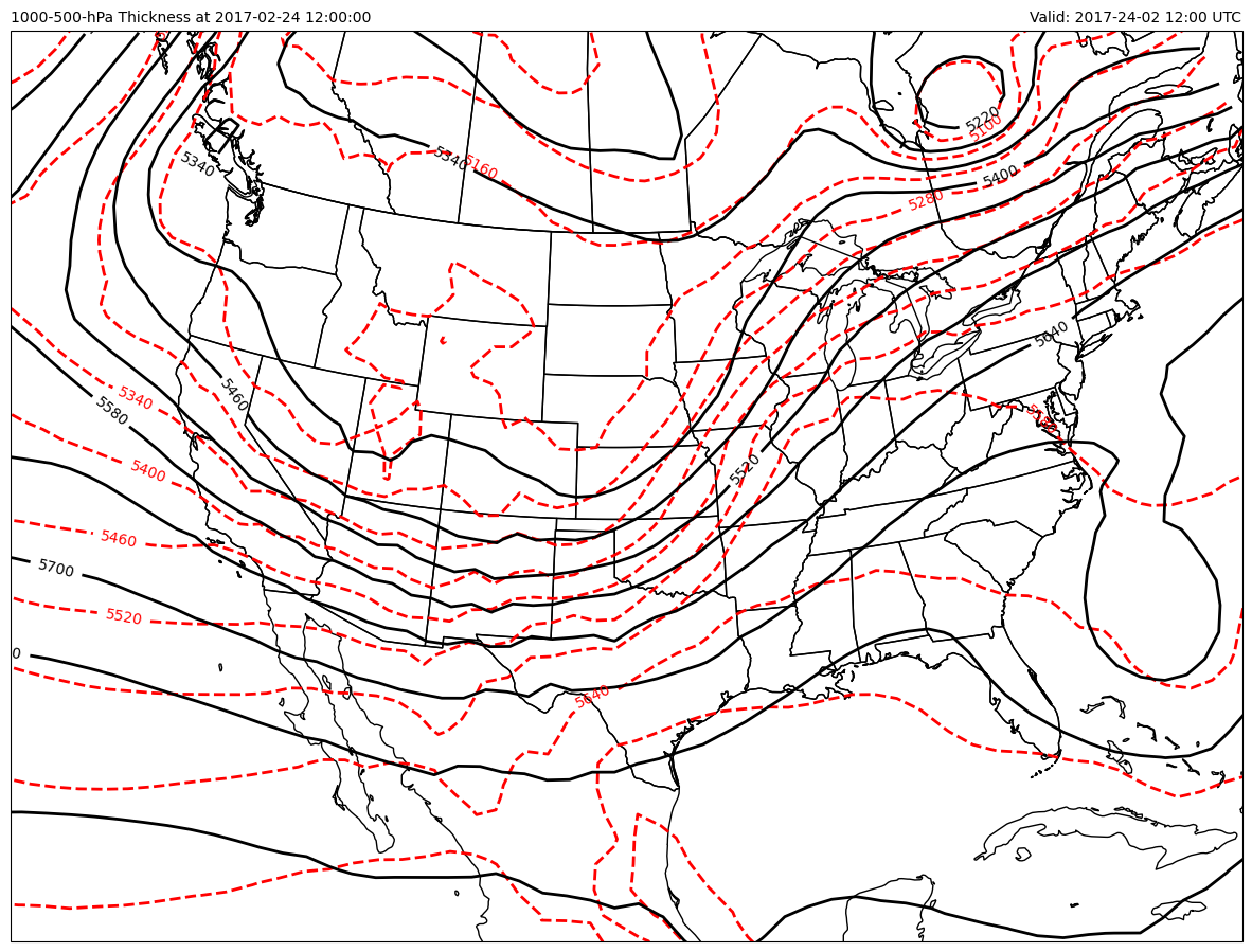
panel.left_title = f'1000-500-hPa Thickness at {date}'
panel.right_title = f'Valid: {date:%Y-%d-%m %H:%M} UTC'
panel.plots = [cntr, cntr2]

# Set the attributes for the panel
# and put the panel in the figure
pc = declarative.PanelContainer()
pc.size = (15, 15)
pc.panels = [panel]

# Show the figure
pc.show()

Note

With this differencing and subsetting by time, we’ll no longer have a time dimension in our variable, so we’ll need to set the time attribute to None.