21.4. Satellite Feature Identification

The entire atmosphere is connected through the temperature and pressure distribution. Changes in the local distribution of temperature can lead to dramatic changes in the structure of the atmosphere, including where we observe strong winds aloft. These areas of strong wind aloft are known as jet streams and they arise due to the temperature differences created between tropical and polar regions in each hemisphere (thermal wind balance). These fast-moving regions of air are a large driver of the speed and motion of mid-latitude cyclones. Therefore, it is important to be able to adequately identify jet streams on upper-level maps as well as satellite images. This section will introduce you to the basic concepts behind jet streams (and fronts to some extent) and how to identify them using satellite imagery.

Jet Streams

There are two main jet streams that affect the North American continent, the polar and subtropical jet streams. The polar jet stream is the northern branch of strong westerly winds aloft and the subtropical jet stream is semi-constant jet stream that straddles with hemisphere around 25–30°N/S. Our main focus will be on the development and identification of the polar jet stream.

A jet stream is the result of the integrated temperature gradient of the atmosphere. Where we observe strong gradients (differences) in temperature at lower-levels of the atmosphere, there will be an area of strong winds aloft. This is a result of the atmosphere being maintained in thermal wind balance, and thus is the explanation for why we have strong winds aloft. Thermal wind balance states that where there are strong temperature gradients in the lower atmosphere, winds will increase with height up to the top of the troposphere (i.e., the tropopause). Inherently this means that where there are jet streams aloft, there are likely fronts at the surface (where the strong temperature gradients are). This links our jets to being key in the evolution of our mid-latitude cyclones.

Jet streams travel with the location of temperature gradients from winter to summer and back again. The strongest temperature gradients over North America occur during the winter months, December, January, and February. The temperature gradient is also at its southernmost extent. Therefore, the jet stream is at its strongest and located on average over the southern half of the United States. As the atmosphere transitions from winter to spring and then to summer, the temperature gradient treks northward and decreases in intensity. This moves the jet stream northward and weakens the overall speed, on average.

On an upper-level map (e.g., 300 hPa) it is rather easy to identify the region of strongest wind by inspecting the plotted wind barbs or contours of wind speed at the level. However, the Earth is primarily covered by our vast oceans where we do not regularly obtain in situ upper-level or surface observations, therefore we must use other tools for identifying the regions of strong winds aloft.

Jet Stream Identification

The most useful satellite image for identifying upper-level flow patterns is the water vapor imagery. Water vapor is ubiquitous throughout the atmosphere, meaning that there is some quantity of water vapor at all times in all places in the atmosphere. This water vapor can then be traced as it circulates within our weather systems around the globe. For jet streams there is a distinct pattern that occurs within water vapor imagery that makes it possible to identify the location of intense jet streams.

Jet streams are located where there is a strong gradient (difference) in moisture on water vapor imagery (Fig. 21.1). This boundary is a result of circulations associated with the jet itself. The jet stream is located parallel to the axis of the boundary as illustrated in Figure 21.1.

Fig. 21.1 Schematic diagram of the water vapor boundary and location of jet streams in relation to those boundaries.

A real example of a jet stream as observed in water vapor imagery is given in Figure 21.2. The main part of the jet stream is located across central California into central Nevada. The sharp boundary in the water vapor imagery indicates southern boundary of the strongest part of the jet stream. Note the contours of wind speed and how they are oriented parallel to that boundary. This real-life example is a cross between the schematic image in Figure 21.1 and 21.3.

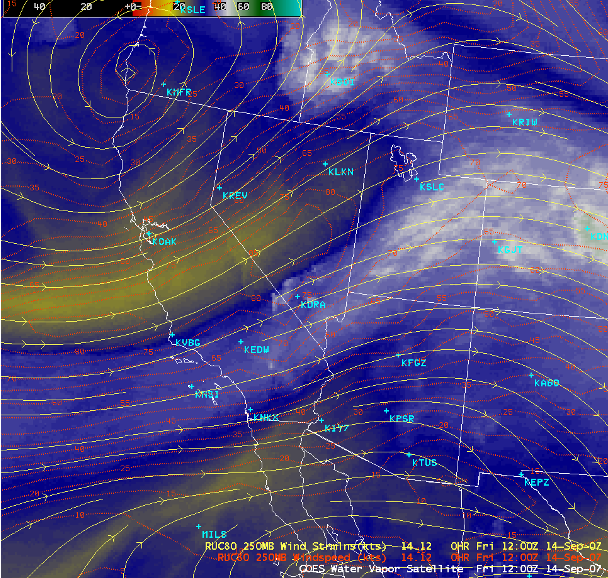
Fig. 21.2 Enhanced water vapor imagery with 250 hPa wind speed analyzed in (kts). Image courtesy of CIMSS at http://cimss.ssec.wisc.edu/goes/blog/wp-content/uploads/2007/09/us_water_vapor_20070914_1200.png

Additionally, a mature mid-latitude cyclone will exhibit the shape of a comma (Figure 21.3). This is the result of airflow through a mid-latitude cyclone. Identifying the stage of cyclone development is key to being able to forecast well in a data sparse region. The use of satellites to identify important features about the mid-latitude cyclone will aid in making a good forecast.

Fig. 21.3 Schematic diagram of a developing mid-latitude cyclone in water vapor imagery with a jet stream.

Wave Pattern

The upper atmosphere is also marked by the wavy pattern of troughs and ridges that is the result of a differentially heated, rotating planet. These waves (a trough/ridge combination) is called a Rossby wave, after the 20^th^ century atmospheric scientist Carl Gustav-Rossby who identified the reason for the wavy pattern. Water vapor can also be used to identify these troughs and ridges by detecting cyclonic (counter-clockwise in the Northern Hemisphere) and anticyclonic (clockwise in the Northern Hemisphere) spin (vorticity) within the motions of the water vapor at upper-levels (Fig. 4).

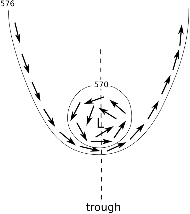
Fig. 21.4 Schematic of a trough aloft and the arrows indicate how the water vapor will rotate around a trough in the Northern Hemisphere.