
20.2. Skew-T Log-p Description#
In the meteorological field, the two most important thermodynamic diagrams are the psuedoadiabatic diagram (also known as a Stüve diagram) and the skew-T/log-P diagram. In this chapter we will focus on the skew-T/log-P diagram. In practice, this diagram is the most widely used thermodynamic diagram in the meteorological discipline.
Similar to surface observations, upper-air observations are encoded into a special format before being transmitted. Historically these radiosonde data were transmitted in three major blocks: TTAA, TTBB, and PPBB. Each of these three blocks has its own significance. TTAA refers to data on the mandatory levels, TTBB refers to data on significant thermodynamic levels, and PPBB refers to significant wind levels. Now they come across in a binary (computer encoded) format. We’ll focus on plotting the vertical profile of the atmosphere that we obtain through the use of radiosondes.
In the Skew-T/Log-p diagram, the logarithm of pressure is used as the vertical (y) axis, with larger values at the bottom. The brown horizontal lines are constant pressure surfaces in units of millibars.
The brown solid lines that tilt toward the upper right are isotherms in °C. Equal distances along the x-axis represent equal differences in temperature, increasing from left to right along the axis. However, the isotherms are tilted toward the upper right rather than running perpendicular to the x-axis. This is why the term “skew” is associated with temperature.
The green dashed lines that tilt with a greater slope to the upper-right are lines of constant mixing ratio in grams of water vapor per kilogram of air. Instead of mixing ratio, some thermodynamic diagrams plot other moisture variables, such as specific humidity. However, in practice, no matter what variable is plotted, the overall meaning and interpretation is the same.
The red solid lines that are oriented perpendicular (or almost perpendicular) to the isotherms are isentropic surfaces, or lines of constant potential temperature in °C. The values of the isentropic surfaces are the same as the temperature lines at 1000 mb. These lines are also known as dry adiabats.
The green curved lines are lines of constant equivalent potential temperature in °C, and are known as pseudoadiabats or moist adiabats. There values are also determined from the temperature at 1000 mb.
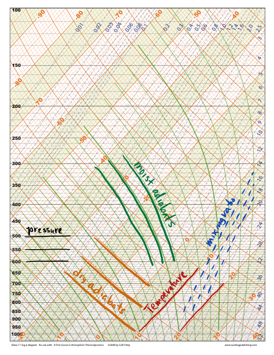
Fig. 20.2 This is an annotated skew-T log-p diagram identifying the important lines that compose the chart.#
Plotting on SkewTs#
Temperature and dew-point temperature are plotted relative to pressure. For a given pressure level, a temperature and dew-point temperature are plotted separately and a line is drawn for both variables that connect the values between reported pressure levels.
The mixing ratio (\(r\)) can be obtained at a given level by interpolating which mixing ratio isopleth intersects the point at which the dew point temperature is plotted.
The saturation mixing (\(r_s\)) ratio can be obtained at a given level by interpolating which mixing ratio isopleth intersects the point at which the temperature is plotted.