Working with NAM Data

This notebook demonstrates plotting gridded NAM data, which has the complication of having winds that are in grid relative coordinates and NOT earth relative. This will entail the need to use some MetPy functionality to easy the plotting of NAM winds.

from datetime import datetime, timedelta, time

from metpy.plots import declarative
from metpy.units import units
import xarray as xr

Get Data

Here we are using current data to demonstrate contour plotting with wind barbs. If you have a different data source you would like to use, simply change out the call to remote data in the open_dataset function to be appropriate for the local or remote data you would like to access. Future chapters will demonstrate different data sources that can be commonly used. Here we’ll use the NAM data from the Unidata THREDDS server.

# Set the date/time of the model run
# The following code will get you yesterday at 12 UTC
yesterday = datetime.utcnow() - timedelta(days=1)
model_run_date = datetime.combine(yesterday, time(12))

# Remote access to the dataset from the UCAR site
ds = xr.open_dataset('https://thredds.ucar.edu/thredds/dodsC/grib'
                     '/NCEP/NAM/CONUS_12km/NAM_CONUS_12km_'
                     f'{model_run_date:%Y%m%d}_{model_run_date:%H%M}.grib2')

Initial Plot

Here let’s plot the data that we get from the NAM. Pay particular attention to the winds barbs relationship to the geopotential height contours.

# Set the plot time with forecast hours
plot_time = model_run_date + timedelta(hours=0)

# Set attributes for plotting contours
cntr = declarative.ContourPlot()
cntr.data = ds
cntr.field = 'Geopotential_height_isobaric'
cntr.level = 300 * units.hPa
cntr.time = plot_time
cntr.contours = range(0, 10000, 120)
cntr.clabels = True

# Add wind barbds
barbs = declarative.BarbPlot()
barbs.data = ds
barbs.time = plot_time
barbs.field = ['u-component_of_wind_isobaric',
               'v-component_of_wind_isobaric']
barbs.level = 300 * units.hPa
barbs.skip = (25, 25)
barbs.plot_units = 'knot'

# Set the attributes for the map
# and put the contours on the map
panel = declarative.MapPanel()
panel.area = 'awips'
panel.layers = ['states', 'coastline', 'borders']
panel.title = f'300-hPa Geopotential Heights at {plot_time}'
panel.plots = [cntr, barbs]

# Set the attributes for the panel
# and put the panel in the figure
pc = declarative.PanelContainer()
pc.size = (12, 12)
pc.panels = [panel]

# Show the figure
pc.show()

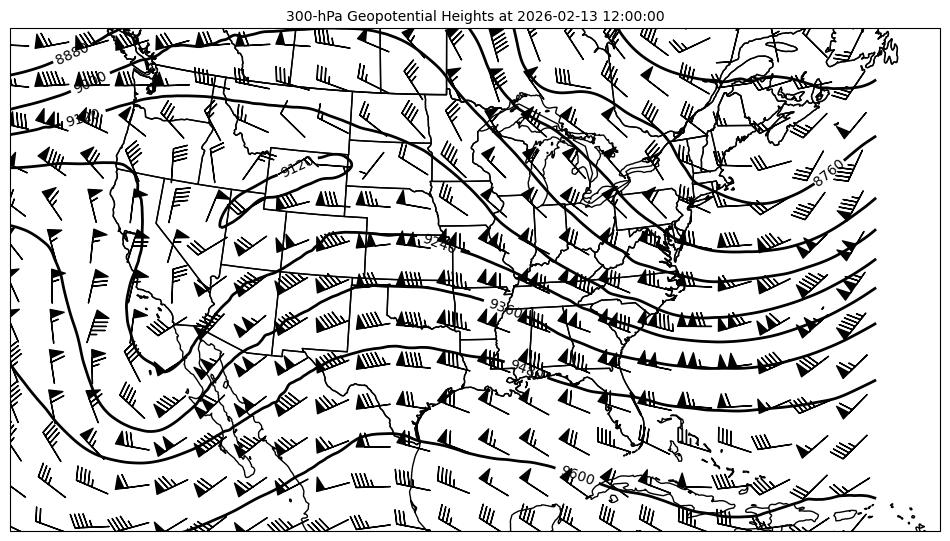
Sanity Check

Here we are plotting 300-hPa geopotential heights and winds. At that level, the winds should be geostrophic, meaning that the winds barbs should be parallel to the contours of geopotential height. When we look toward the edge of the map this is where we see that the wind barbs are not clearly conforming to geostrophic balance. The winds are crossing the geopotential height contours at an angle that they shouldn’t be. This behaviour is due to the curvature of the projection not aligning with the assumptions made to plot the wind barbs.

Luckily we have an easy solution built in to the MetPy declarative syntax to convert the stored grid relative winds and make them earth relative for plotting. The attribute to set as part of the BarbPlot() class is earth_relative. We need to tell MetPy that our winds are NOT earth relative. This is a boolean setting, such that for our NAM winds earth_relative should be set to False.

Corrected NAM Winds

Let’s try it out and compare the NAM wind barbs that are grid-relative to our recomputed earth relative wind barbs using the MetPy attribute.

# Set the plot time with forecast hours
plot_time = model_run_date + timedelta(hours=0)

# Set attributes for plotting contours
cntr = declarative.ContourPlot()
cntr.data = ds
cntr.field = 'Geopotential_height_isobaric'
cntr.level = 300 * units.hPa
cntr.time = plot_time
cntr.contours = range(0, 10000, 120)
cntr.clabels = True

# Add wind barbds
barbs = declarative.BarbPlot()
barbs.data = ds
barbs.time = plot_time
barbs.field = ['u-component_of_wind_isobaric',
               'v-component_of_wind_isobaric']
barbs.level = 300 * units.hPa
barbs.skip = (25, 25)
barbs.plot_units = 'knot'

# Add wind barbds
barbs2 = declarative.BarbPlot()
barbs2.data = ds
barbs2.time = plot_time
barbs2.field = ['u-component_of_wind_isobaric',
               'v-component_of_wind_isobaric']
barbs2.level = 300 * units.hPa
barbs2.skip = (25, 25)
barbs2.plot_units = 'knot'
barbs2.color = 'tab:red'
barbs2.earth_relative = False

# Set the attributes for the map
# and put the contours on the map
panel = declarative.MapPanel()
panel.area = 'awips'
panel.layers = ['states', 'coastline', 'borders']
panel.title = (f'300-hPa Geopotential Heights at {plot_time}\n'
               'grid-relative wind barbs (black) and earth-relative wind barbs (red)')
panel.plots = [cntr, barbs, barbs2]

# Set the attributes for the panel
# and put the panel in the figure
pc = declarative.PanelContainer()
pc.size = (15, 15)
pc.panels = [panel]

# Show the figure
pc.show()

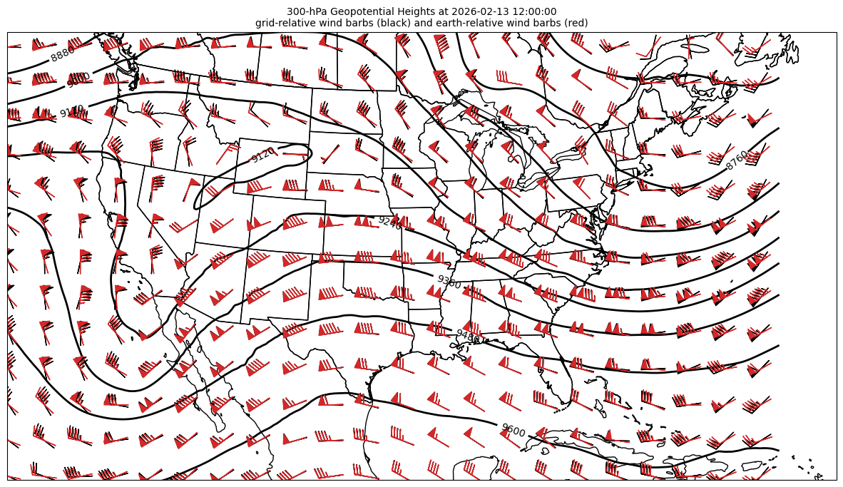
In the above graphic we can observe the corrected winds (in red) and notice that the largest differences are noted on the edges of the map where the curvature of the projection is notably different between the projection of the winds and the projection of the plot. The only change that was needed to get the winds in the correct orientation was to set the attribute earth_relative to False since the NAM output stores wind components in a grid-relative format.