20.10. Advanced Skew-T Calculations and Plotting

This notebook demonstrates calculating a number of common sounding parameters and plotting some of them on a skew-T diagram.

Import Packages

from datetime import datetime

import matplotlib.pyplot as plt
import metpy.calc as mpcalc
from metpy.plots import SkewT
from metpy.units import units, pandas_dataframe_to_unit_arrays
import numpy as np
from siphon.simplewebservice.wyoming import WyomingUpperAir

Get Data

# Set date that you want
# Data goes back to the 1970's
date = datetime(2007, 5, 4, 18)

# Set station ID, there are different stations back in the day
# Current station IDs found at http://weather.rap.ucar.edu/upper
station = 'DDC'

# Use Siphon module to grab data from remote server
df = WyomingUpperAir.request_data(date, station)

20.11. Subsetting Data

When performing calculations on radiosonde data it is best to subset the data to only use the data needed, which is typically pressures >= 100 hPa. This can be accomplished via code by creating a Boolean (true/false) array from a simple inequality and then using that array to subset all of the variable arrays.

# Create dictionary of unit arrays
data = pandas_dataframe_to_unit_arrays(df)

# Isolate united pressure array from dictionary
p = data['pressure']

# Setting a subset to only use the data needed
idx = p.m > 99

# Isolate united arrays and subset from dictionary
p = p[idx]
T = data['temperature'][idx]
Td = data['dewpoint'][idx]
u = data['u_wind'][idx]
v = data['v_wind'][idx]

Calculation of Sounding Parameters

Once we have our data, we can calculate any of the skew-T variables we desire, such as LCL using the functions available in MetPy (https://unidata.github.io/MetPy/latest/api/generated/metpy.calc.html#soundings).

Lifting Condensation Level

This is the level at which a lifted parcel will become saturated (e.g., have 100% RH). The function in MetPy is called lcl and takes inputs of pressure, temperature, and dewpoint.

MetPy LCL Documentation

This function will output two values, the first is the pressure level of the LCL and the second is the temperature of the LCL.

# Calculate LCL pressure and temperature
# Note: since lcl function returns two values, we can have
# two variables to the left of the equal sign

lcl_pressure, lcl_temperature = mpcalc.lcl(p[0], T[0], Td[0])
print(f'LCL: {lcl_pressure:.2f}')

LCL: 849.75 hectopascal

Parcel Profile

The parcel path is essential the temperature that a parcel would have if lifted from a given level. This is an essential component to determining the stability of the atmosphere (a la introduction to meteorology) and determining the available energy for thunderstorm production.

MetPy Parcel Profile Documentation

The input would be all of the pressures from the sounding and the starting temperature and dewpoint values for where the parcel is being lifted from. Typically, this is the zeroth element since we want to lift a surface parcel.

# Calculate full surface parcel profile and add to plot as black line
prof = mpcalc.parcel_profile(p, T[0], Td[0]).to('degC')

CAPE/CIN

Often, we want to know how much energy might be available for use in the generation of thunderstorms, so we want the ability to calculate CAPE. This is actually not a trivial calculation due to any number of details that could be considered, but it is not too hard to do a basic estimation that works well for forecasting purposes. Along with CAPE, we get CIN or convective inhibition, a measure of the excess amount of energy we need to be able to realize any CAPE that might be present in a profile. MetPy has a function that computes both of these values using a trapezoid integration scheme (and you thought you would never hear about estimating an integral outside of calculus!?!).

MetPy CAPE/CIN Documentation

Here our inputs expand to four items, pressure, temperature, dewpoint, and the parcel profile. Each variable must contain the same number of points corresponding to all of the pressure levels given in the dataset.

# Calculate the CAPE and CIN of the profile
cape, cin = mpcalc.cape_cin(p, T, Td, prof)

print(f'CAPE: {cape:.2f}')
print(f'CIN: {cin:.2f}')

CAPE: 2032.69 joule / kilogram
CIN: -126.51 joule / kilogram

Lifted Index

The LI is the difference between the parcel temperature and environmental temperature at 500 hPa. If you have calculated the parcel profile, then this becomes a simple difference of two values once you have found both values at 500 hPa.

MetPy Lifted Index Documentation

Here we need to feed the function the pressure, temperature, and parcel profile temperature.

# Compute LI and print result
LI = mpcalc.lifted_index(p, T, prof)
print(f'LI: {LI[0].m:.02f} C')

LI: -6.18 C

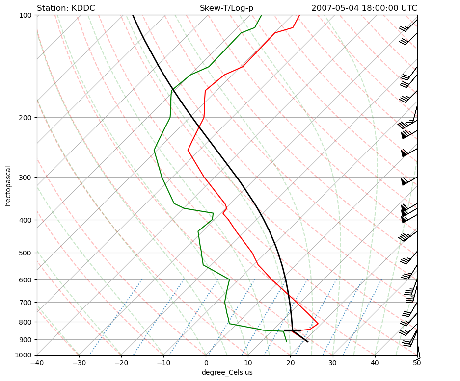
Plot Skew-T with Parcel Path

A common thing to plot on a skew-T image is the parcel path, this allows a meteorologist to visually estimate the amount of CAPE and CIN since the area on a skew-T is directly proportional to energy. The key area being between the environmental temperature and the parcel profile.

Plotting the parcel profile is pretty easy, we can use the same skew.plot to plot on the same axis and use our pressure and profile temperature to plot the parcel profile line. In the code below we are plotting the parcel path in black with a thicker line than normal.

The LCL is also highlighted with a straight line at the pressure level at which our parcel becomes saturated.

# Plot a skew-T image
fig = plt.figure(figsize=(10, 10))

# Set up the skewT axes
skew = SkewT(fig,  rotation=45)

# Plot the data using normal plotting functions, in this case using
# log scaling in Y, as dictated by the typical meteorological plot
skew.plot(p, T, 'r')
skew.plot(p, Td, 'g')

# Plot barbs skipping to every other barb
skew.plot_barbs(p[::2], u[::2], v[::2], y_clip_radius=0.03)

# Set sensible axis limits
skew.ax.set_ylim(1000, 100)
skew.ax.set_xlim(-40, 50)

# Plot the skew-T parcel temperature profile
skew.plot(p, prof, 'k', linewidth=2)

# Plot a line marker at the LCL level
skew.plot(lcl_pressure, lcl_temperature, '_', color='black', markersize=24, 
          markeredgewidth=3, markerfacecolor='black')

# Add the relevant special lines
skew.plot_dry_adiabats(t0=np.arange(233,555,10)*units.K, alpha=0.25)
skew.plot_moist_adiabats(colors='tab:green', alpha=0.25)
skew.plot_mixing_lines(colors='tab:blue', linestyle='dotted')

# Plot some titles
plt.title(f'Station: K{station}', loc='left')
plt.title('Skew-T/Log-p', loc='center')
plt.title(f'{date} UTC', loc='right')

# Show the plot
plt.show()

# Save the plot by uncommenting the following line
#plt.savefig('advanced_skewt_image.png', bbox_inches='tight', dpi=150)