The Influence of SST on Midlatitude Cyclones

There are many factors that can influence the the life cycle of a midlatitude cyclone. For cyclones that form and track along coastal regions of the southern and eastern US, sea surface temperatures (SSTs) can have a profound impact on the strength and speed of intensification of a given cyclone. In order to begin to understand the relationship we’ll want to look at data that represent both the atmospheric strength of a cyclone with some information about ocean conditions. Where we have warmer SSTs there is greater capacity for moisture just above the ocean surface, which in turn can lead to greater latent heat release. It’s the latent heat release that can strongly modify the environment to amplify atmospheric processes and thus produce a deeper (stronger) midlatitude cyclone in a very short amount of time.

Let’s investigate a case to determine whether SSTs appear to play a major role in the life cycle of a midlatitude cyclone.

Case: March 2023 Nor’Easter Dates: 11-15 March 2023

Main Impacts: Heavy Snowfall, High Winds, Blizzard Conditions

States Impacted: New York, Massechusettes

Background Resource Information

Atmospheric Data

There are any number of different datasets that can be used to access atmospheric data. Here we are going to access the National Oceanic and Atmospheric Administration (NOAA) National Center for Environmental Information (NCEI) THREDDS server to gather Global Forecast System analysis output to capture the strength of the midlatitude cyclone using the variable that gives the MSLP.

Data Source: GFS 0.5 Degree Analysis Files

from datetime import datetime

from metpy.units import units
import xarray as xr

# Specify our date/time of product desired
date = datetime(2023, 3, 11, 12)

# ds = xr.open_dataset('https://thredds.rda.ucar.edu/thredds/dodsC/files/g/ds084.1/'
#                      f'{date:%Y}/{date:%Y%m%d}/gfs.0p25.{date:%Y%m%d%H}.f000.grib2')
ds = xr.open_dataset('https://www.ncei.noaa.gov/thredds/dodsC/model-gfs-g4-anl-files/'
                     f'{date:%Y%m/%Y%m%d}/gfs_4_{date:%Y%m%d_%H}00_000.grb2')
# Subset data to be just over the CONUS
ds = ds.sel(lat=slice(80, 10), lon=slice(360-145, 360-40))

Ocean Data

There are also a number of different data sources that can provide information about the sea surface temperatures (SSTs) of the ocean and large freshwater bodies (e.g., the Great Lakes). Here access to a THREDDS-like server will allow us to gather Optimal Interpolation (OI) SST that contains both the actual SST values as well as the anaomalies from long term means already computed.

Data Source: https://coastwatch.pfeg.noaa.gov/erddap/griddap/ncdcOisst21NrtAgg.html

ds_sst = xr.open_dataset('https://coastwatch.pfeg.noaa.gov/erddap/griddap/ncdcOisst21NrtAgg')

ds_sst = ds_sst.metpy.sel(time=date, method='nearest').sel(latitude=slice(10, 80), longitude=slice(360-145, 360-40))

print(f"Nearest SST time: {ds_sst.time.values.astype('datetime64[ms]').astype('O')}")

Nearest SST time: 2023-03-11 12:00:00

Visualize Combined Data

For this case we are looking to assess the potential role that SSTs had in the evolution of the midlatitude cyclone. The impact that would be made would occur through the latent heat release that would be amplified due to the cyclone moving across relatively warmer SSTs compared to the cold air moving off the land. The addition of this latent heat release would amplify the amount of rising motion that couple aid in making the storm stronger (deeper; with a lower surface pressure) than would have happened if the storm occurred only over land.

Let’s investigate both the actual SST values and the SST anomaly values to assess the possible impact on the cyclone evolution.

Plot SST and MSLP Data

from metpy.plots import declarative
import numpy as np

sst = declarative.RasterPlot()
sst.data = ds_sst
sst.field = 'sst'
sst.colormap = 'RdYlBu_r'
sst.colorbar = 'horizontal'
sst.image_range = (-5, 35)

mslp = declarative.ContourPlot()
mslp.data = ds
mslp.field = 'Pressure_reduced_to_MSL_msl'
mslp.time = date
mslp.contours = range(0, 2000, 4)
mslp.plot_units = 'hPa'
mslp.smooth_field = 2
mslp.clabels = True

# Panel for plot with Map features
panel = declarative.MapPanel()
panel.layout = (1, 1, 1)
panel.projection = 'area'
panel.area = 'ehlf'
panel.layers = ['coastline', 'borders', 'states']
panel.left_title = f'SST (C) and MSLP'
panel.right_title = f'Valid: {date} UTC'
panel.plots = [sst, mslp]

# Bringing it all together
pc = declarative.PanelContainer()
pc.size = (10, 12)
pc.panels = [panel]

pc.show()

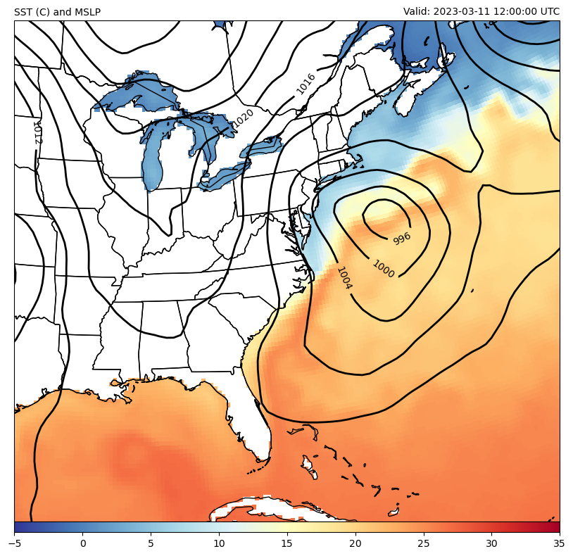
SST and MSLP Analysis

In the above image we plotted, there appears to be “warm” sea surface temperatures (SSTs) underneath the developing and moving cyclone. The Gulf Stream is bringing the warm surface water from southern latitudes along the Atlantic coast. The SST values are between 20-25C, which is fairly warm for March and would likely be helping the cyclone to be stronger due to the resultant latent heat release.

But how do we know that these are warm SST values for March? This is where it would be useful to look at the SST anomaly values to assess if the temperatures are in fact a little or a lot warmer than a thirty year average.

Plot SST Anomaly and MSLP Data

sst = declarative.RasterPlot()
sst.data = ds_sst
sst.field = 'anom'
sst.colormap = 'coolwarm'
sst.colorbar = 'horizontal'
sst.image_range = (-13, 13)

mslp = declarative.ContourPlot()
mslp.data = ds
mslp.field = 'Pressure_reduced_to_MSL_msl'
mslp.time = date
mslp.contours = range(0, 2000, 4)
mslp.plot_units = 'hPa'
mslp.smooth_field = 2
mslp.clabels = True

# Panel for plot with Map features
panel = declarative.MapPanel()
panel.layout = (1, 1, 1)
panel.projection = 'area'
panel.area = 'ehlf'
panel.layers = ['coastline', 'borders', 'states']
panel.left_title = f'SST Anom. (C) and MSLP'
panel.right_title = f'Valid: {date} UTC'
panel.plots = [sst, mslp]

# Bringing it all together
pc = declarative.PanelContainer()
pc.size = (10, 12)
pc.panels = [panel]

pc.show()

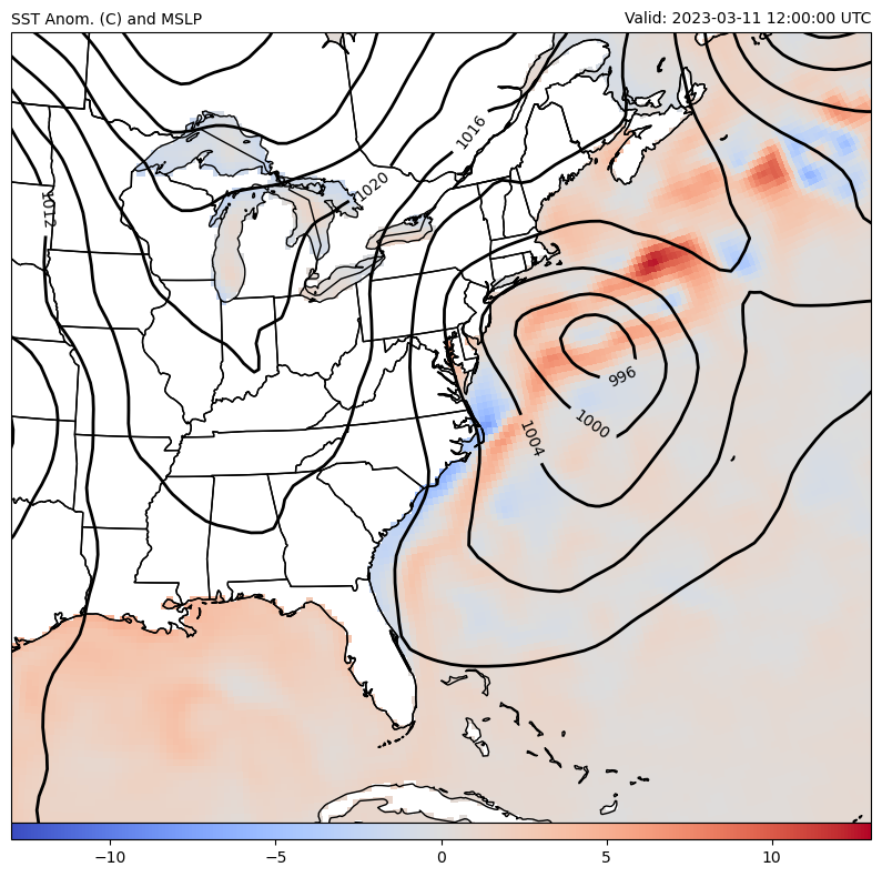
SST Anomaly and MSLP Analysis

In the above figure, we get a more nuanced insight into the seasonal nature of the SST values. There are regions surrounding the midlatitude cyclone that are quite a bit warmer than the 30 year average, but also some areas that are slightly cooler. Of particular note is that just to the north of the cyclone - its likely direction of motion - is a strip of warmer than average SSTs, but not where we had the warmest SSTs overall. This is interesting because while the water is colder, its not as cold is it would normally be, thus likely enhancing the latent heat release effect during this cyclones life cycle.

Conclusion

In this analysis we have only investigated a single time to compare the SSTs and SST anomalies with the observed MSLP of a developing midlatitude cyclone. From the data, it appears likely that the warm SSTs along the Atlantic coast were at least partially responsible for the overall strength of the deepening cyclone. It would be better to analyze multiple times to observe the full evolution of the cyclone and note any changes in the SSTs as it move up the Atlantic seaboard.